This is a repo that represents our classwork and some notes on the bellman equation. Feel free to use this as you see fit.

Table of Contents

1. Bellman Equation
2. Big O Notation
3. Knapsack Problem
   • State Space
   • Action Space
   • Transition Function
   • Reward/Immediate Value Function
   • Terminal Case

Bellman Equation

Formally the bellman equation is $V(s) = \underset a{max} R(s,a) + V(s')$

• s := our state
• a := our action
• V := is the optimal value function. It is a magical function that always find the maximum value in the long run. If it makes you happy you can represent it as $V_{max}$
• $s'$ := our new state that is reached when we perform action $a$ on state $s$. We can think of $s' = T(s,a)$ where $T$ is our transition function.
• R(s,a) := immediate reward function. Also known as Immediate Value Function. This will vary problem to problem.

In english, we can calculate the maximum value for the entire problem starting at state $s$ by choosing the a that maximizes our V function.

Our V function is going to be the sum of our current/immediate reward function and our projected future rewards.

Our future rewards is represented by $V(s')$ where $s'$ is the new state we reach when we take action a

You will notice that this equation is recursive and will go on forever if we let it because there will always be a new state. We must define some $s_{term}$ such that there is no $s'$ within the action space.

$V(s_{term}) = R(s_{term},a)$

Big O Notation and Runtime Complexity

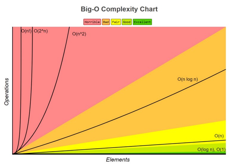
In class we discussed the concept of runtime complexity. In essence, runtime complexity is how much longer your program will take to finish as we make it bigger. If your problem is 3 times as big now, by what factor will your runtime grow?

Here is a pretty good link that explains the concept of big O. You won't have to use this ever, but its good to know

Formal definition of Big O

$g(x) = O(f(x)) \iff \exists$ $n,a$ s.t

$\forall$ $x >n, \quad a \cdot f(x)> g(x)$

If we look at the math behind this statement, it means we can always pick out sufficiently large values for and n so that f serves as an upper bound of g.

This is similar to the concept of limits that you may have encountered in calculus. Just like limits, you can pretty much just look at the "biggest" term and pay attention to that.

This means that f(x) serves as a conceptual upper bound for g(x). Rather than talking about some very specific functions we can very easily communicate just about how fast (or slow) our program will be.

Big O	Example
O(1)	normal operations (=, +, -, *,/,**)
O(log(n))	searchign for things when they've been organized in groups
O(n)	for loops
O(nlog(n))	organizing things into groups and then searching for an item
O(n^2)	double nested for loops
O(n^3)	triple nested for loops
O(n^4)	quad nested for loops
O(2^n)	Branching operations. Usually recursive or forking calls
O(n!)	More complex combinatorial checks

Most problems that we will be interested in this class will be $O(2^n)$. This makes it really important for us to solve them as efficiently as possible.

Knapsack Problem

In the knapsack problem we pretend like we are a robber. We sneak into the castle and have a choice to steal or not to steal. The caveat is that we have a limited amount of space in our knapsack. How do we pick the best combination of items?

Lets take a look at our information

Item Idx	Weight	Value
0	$w_0$	$v_0$
1	$w_1$	$v_1$
2	$w_2$	$v_2$
3	$w_3$	$v_3$
...	...	...
n	$w_n$	$v_n$

Lets define $\alpha_i$ as our decision to take or leave item $i$. 1 for take and 0 for leave.

Our objective becomes $\Pi = \sum_{i=0}^n \alpha_i \cdot v_i$

with respect to our constraint of maximum weight $W$.

$W \geq \alpha_i \cdot w_i$

Action Space

Our action space is as defined above. Every single item we can either take or not take. 0 or 1 for every state. Easy peasy. Sometimes we will have different action spaces dependent on our current state

State Space

Our state space is more nuanced. Remember state functions don't care about the past. They only care abou thte present and in Dynamic Programming we care about the future. So our state space should capture some of this information.

Our state should also give us information about the subproblem. We need this to have our nice little recursive relationship. These can be pretty tricky to define, but once you get the hang of it, there's no stopping you.

In our case we care about what item index we are currently making a decision about and how much weight is remaining from our maximum. If we are at item 4 with a remaining weight of 20 our future value will not affected by our decisions for items 0-3 (though our cummulative value will be.)

Transition Function

What happens when we add an item to our bag? Well our bag gets heavier and closer to our carrying capacity. That means we have less remaining weight in our bag. We have also made a decision about our current item, so it's time to move on to our next item.

What happens when we decide not to add an item? Well our carrying capacity is unaffected, but we shouldn't make two decisions on that item so we should move onto the next one.

Reward/Immediate Value Function

Our reward function is the amount that our cumulative total increases as a result of our action.

How much does our total reward $\Pi$ increase when we make a choice $\alpha$ scroll up and check it out.

The answer is $\alpha_i \cdot v_i$

Terminal Case

When are we done with the problem? We have two cases right?

1. We are out of weight
2. We are out of items in either case there is no need to update our state and keep going with these recursive calls. Our value for all future periods will be 0.

This is all the information we need to implement.