Building a Neural Network

This project aims at creating a neural network from scratch, to apprehend not only the theoretical part but also the practical part.

Table of Contents

1. Introduction

   1.1. Why build a Neural Network from scratch?

   1.2. What is the goal of this project?

2. Neural Network notions

   2.1. Neural Network

   2.2. Notations

   2.3. Activation Function

   2.4. Feed-forward

   2.5. Loss Function

   2.6. Backpropagation

3. Implementing and testing

4. Performance Metrics

5. First batch of results

6. Optimization

7. Conclusion

Introduction

Why build a Neural Network from scratch?

I'm really into data and AI, so I chose to work on data science projects on the side. Among the algorithms to learn are neural networks. I believe that building a neural network from scratch is a great way to understand how it works. It allows you to apprehend the theoretical part but also the practical part. It is a great way to understand the different components of a neural network and how they interact with each other. Then, explaining the code to someone else is a great way to consolidate the knowledge acquired. So I hope the documentation will be clear enough for you to understand how to build a NN. That would mean I'm not too bad at it! ^^

What is the goal of this project?

The goal of this project is to build a neural network from scratch, that meets the following expectations:

Requirements:

The neural network must be able to:

• take any number of inputs
• have any number of hidden layers
• have any number of neurons in each hidden layer
• have any number of outputs
• use any activation function
• use any loss function

Constraints:

The neural network must use the following algorithm:

• backpropagation algorithm

To summarise the goal of this project, I want to build a neural network that is as modular as possible, while using the most common algorithms in the field of neural networks.

Neural Network notions

In this section, I will explain the different notions that are important to understand when building a neural network.

Here's an example of what a neural network looks like :

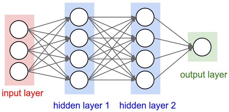
Source of image: PyImageSearch

Neural Network

A neural network is a set of algorithms, modeled after the human brain, that is designed to recognize patterns. It is composed of layers of neurons, each of which applies an activation function to the weighted sum of its inputs. These layers are divided into three types:

• the input layer, which receives the input data. The number of nodes of the input layer must match the number of features of the input data.
• the hidden layers, which process the data
• the output layer, which produces the output data, and therefore, the predictions. The idea is to do a forward pass, where the input data is passed through the network, and the output is predicted. Then, the neural network uses a loss function to measure the difference between the predicted output and the actual output. The goal is to minimize this difference by adjusting the weights of the neurons. This is done through the backpropagation algorithm, which calculates the gradient of the loss function with respect to the weights and biaises of the neurons, and updates the weights/biaises accordingly. Finally, we can train the neural network by repeating the forward pass and the backpropagation algorithm until the loss function is minimized.

The training process is usually divided into several steps:

• The first step consists in splitting the data into a training set and a test set.
• The second step consists in normalizing the data, to make it easier for the neural network to learn.
• The third step consists in initializing the weights and biaises of the neurons.
• The fourth step consists in training the neural network on the training set, by doing a forward pass and a backpropagation algorithm.
• The fifth step consists in evaluating the neural network on the testing set, to see how well it generalizes to new data.
• The sixth step consists in tuning the hyperparameters of the neural network, to improve its performance.

Notations

In order to build a neural network, we need to define the following notations:

• nb_layers: the number of layers of the neural network.

• nb_neurons: the list of the number of neurons in each layer of the neural network, which is a list of integers of length nb_layers. The value of n[0] is the number of features of the input data X.

• g: the activation function of the neural network.

• X: the input data, which is a matrix of shape (n, m), where n is the number of features and m is the number of samples.

• y: the actual values of the input data.

• W: the list of weight matrices of the neural network, which is a list of matrices of shape (n[i], n[i-1]), where n[i] is the number of neurons in the i-th layer of the neural network, and n[i-1] is the number of neurons in the (i-1)-th layer of the neural network.

• b: the list of bias vectors of the neural network, which is a list of vectors of shape (n[i], 1), where n[i] is the number of neurons in the i-th layer of the neural network.

• Z: the list of weighted sums of the neural network (to which are added the biaises), which is a list of matrices of shape (n[i], m), where n[i] is the number of neurons in the i-th layer of the neural network, and m is the number of samples.

• A: the list of output matrices of the neural network, which is a list of matrices of shape (n[i], m), where n[i] is the number of neurons in the i-th layer of the neural network, and m is the number of samples. The value of A[0] is the input data X. The difference between A and Z is that A is the output of the activation function applied to Z.

• $\hat{Y}$: the prediction of the neural network, which is the output of the output layer of the neural network.

Activation Function

An activation function is a mathematical function that is applied to the weighted sum of the inputs of a neuron, to introduce non-linearity into the neural network.

There are several activation functions that can be used in a neural network. The most common ones are:

• the Sigmoid Function

  Use Case: Output layer of a binary classification model.

$$ \sigma(x) = \frac{1}{1 + e^{-x}} $$

• the Tanh Function

  Use Case: Often preferred in hidden layers when inputs can be negative.

$$ \tanh(x) = \frac{e^x - e^{-x}}{e^x + e^{-x}} $$

• the ReLU Function

  Use Case: Very commonly used in hidden layers for deep networks.

$$ f(x) = \max(0, x) $$

• the Leaky ReLU Function

  Use Case: A variant of the ReLU function that allows a small gradient when the input is negative.

$$ f(x) = \max(0.01x, x) $$

• the Softmax Function

  Use Case: Output layer of a multi-class classification model.

$$ \sigma(z_i) = \frac{e^{z_i}}{\sum_{j} e^{z_j}} $$

In order to build a neural network, we have to choose an activation function. First we will build it using the sigmoid function. It is set as default function, but the idea is for the code to be modular, so in the end it should be possible to choose the activation function.

Feed Forward

The feed-forward algorithm is the process of passing the input data through the neural network, from the input layer to the output layer, to make a prediction.

The feed-forward algorithm goes like follows:

• The input data is passed through the input layer, and the output of the input layer is passed to the first hidden layer.
• The output of the first hidden layer is passed to the second hidden layer, and so on, until the output layer.
• The output of the output layer is the prediction of the neural network.

The feed-forward algorithm is the first step of the training process of a neural network. It allows the neural network to make a prediction, which can be compared to the actual output to calculate the loss function.

Our input data is a matrix of shape (n, m), where n is the number of features and m is the number of samples. This matrix will be defined as the X matrix.

The value of A[0] is the input data X. We define the value of Z[i] as the weighted sum of the inputs of the i-th layer of the neural network, to which we add the bias of the i-th layer. The value of Z[i] is calculated as follows:

$$ Z[i] = W[i-1] \cdot A[i-1] + b[i] $$

Where:

• W[i-1] is the weight matrix of the links between the (i-1)-th and the i-th layer of the neural network.
• A[i-1] is the output of the (i-1)-th layer of the neural network.
• b[i] is the bias vector of the i-th layer of the neural network.

The value of A[i] is the output of the i-th layer of the neural network, after applying the activation function to the value of Z[i]. The value of A[i] is calculated as follows:

$$ A[i] = g(Z[i]) $$

Where:

• g is the activation function of the i-th layer of the neural network.

The value of A[i] is the output of the i-th layer of the neural network.

Finally, the value of $\hat{Y}$ is the output of the output layer of the neural network, which is the prediction of the neural network. The value of $\hat{Y}$ is calculated as follows:

$$ \hat{Y} = A[L] $$

Where:

• L is the number of layers of the neural network.
• A[L] is the output of the output layer of the neural network.

To build the feed-forward algorithm, we need to define the following functions:

• the init_layers function, which initializes the weights and biaises of the neural network. It takes as input the number of required layers of the neural network, and the number of neurons in each layer of the neural network, and returns both the lists of weight matrices and bias vectors of the neural network.
• the feed_forward function, which applies the feed-forward algorithm to the neural network. It takes as input the input data X, the number of layers required, the number of neurons in each layer of the neural network. This enables the function to call the init_layers function to initialize the weights and biaises of the neural network. The function also takes as input the activation function to be used in the neural network. The default activation function is the sigmoid function. Finally, the function returns the list of A matrices, Z matrices, and the prediction of the neural network. Theoretically, the A and Z lists should not be returned, but they are useful for debugging purposes.

These functions are tested in the nnTesting.ipynb notebook. They are first tested on specific examples, and then generalized through random examples.

The feed-forward algorithm is the first step of the training process of a neural network. It allows the neural network to make a prediction, which can be compared to the actual output to calculate the loss function.

Loss Function

In this section, we shall provide several loss functions, useful depeneding on the use cases. These functions are used to measure the difference between the predicted output of the neural network and the actual output. The goal is to minimize this difference by adjusting the weights and biaises of the neurons.

It is important to choose convex functions, as local minimums can be a problem. Indeed, the backpropagation algorithm is based on the gradient of the loss function, and if the loss function has local minimums -which non convex functions may have-, the algorithm may get stuck in them. This would imply that the neural network would not be able to learn the optimal weights and biaises. The predictions of the neural network would not be as accurate as they could be.

The most common loss functions are:

• the Mean Squared Error Loss Function

  Use Case: Regression problems.

$$ L(\hat{Y}, Y) = \frac{1}{m} \sum_{i=1}^{m} (\hat{Y} - Y)^2 $$

• the Binary Cross Entropy Loss Function

  Use Case: Binary classification problems.

$$ L(\hat{Y}, Y) = - \frac{1}{m} \sum_{i=1}^{m} Y \log(\hat{Y}) + (1 - Y) \log(1 - \hat{Y}) $$

Now that we have defined the loss functions, we can build the backpropagation algorithm, which is the second step of the training process of a neural network. It allows the neural network to adjust the weights and biaises of the neurons, to minimize the loss function.

Backpropagation

The backpropagation algorithm is the process of calculating the gradient of the loss function with respect to the weights and biaises of the neurons, and updating the weights and biaises accordingly.

The backpropagation algorithm goes like follows:

• The gradient of the loss function with respect to the weights and biaises of the output layer is calculated.
• The gradient of the loss function with respect to the weights and biaises of the hidden layers is calculated, by using the chain rule.
• The weights and biaises of the neurons are updated, by subtracting the gradient of the loss function with respect to the weights and biaises of the neurons, multiplied by the learning rate.

Backpropagation implementation

The backpropagation algorithm is implemented in the backpropagation function. The function is strictly modular, as it takes as input the number of layers of the neural network, the number of neurons in each layer of the neural network, the lists of weight matrices and bias vectors of the neural network, the lists of A and Z matrices of the neural network, the prediction of the neural network, the actual output, the learning rate, and the activation function. The function returns two lists : grad_W and grad_b. These lists contain the gradients of the loss function with respect to the weights and biaises of the neurons, respectively. Then, the update_parameters function is called to update the weights and biaises of the neurons.

The backpropagation step of building a neural network is easily the most complex part of the process. It is the step where the neural network learns from the data, and adjusts its weights and biaises to minimize the loss function. It is the step where the neural network becomes more accurate, and is able to make better predictions. This means testing is essential here. There are several ways to test the backpropagation algorithm.

• The most common way is to use the gradient checking method. This method consists in comparing the gradients calculated by the backpropagation algorithm with the gradients calculated by the finite difference method. If the gradients are close enough, then the backpropagation algorithm has good chances of being correct. If not, then the backpropagation algorithm needs to be fixed. We will calculate the relative error between the gradients calculated by the backpropagation algorithm and the gradients calculated by the finite difference method. A good threshold for the relative error is $10^{-7}$.

• Another way to test the backpropagation algorithm is to do an overfitting test. This test consists in training the neural network on a very small dataset, and checking if the loss function decreases with a big number of epochs. If the loss function decreases, then the backpropagation algorithm is working. If not, then the backpropagation algorithm needs to be fixed.

Implementing and testing

The implementation consists of the following functions:

init_layers:

Argument n°	Argument Name	Argument description
1	nb_layers	Number of layers within the neural network (including both the input and output layers). There may be some changes to automatise the input layer later in the project
2	nb_neurons	List of the number of neurons per layer. It includes both the input and output layers once again. Example: if nb_neurons[1] = 3, there will be 3 neurons in the first hidden layer of the NN.

Return variable n°	Variable Name	Variable description
1	W	Initialised list of Weight matrices. Default initialisation is Normal Xavier. The matrices are of shape (nb_neurons[i+1], nb_neurons[i]) for a giver layer i
2	b	The list of initialised biais matrices. They are all set to 0. It is important to note that the values themselves do not matter much, as long as they are all the same. The matrices are of shape (nb_neurons[i], 1).

NB: At first, we initialised weights with random values with the np.random.randn. But when it is done with a sigmoid, which is our default activation function, this can be problematic. Indeed, the randn function generates an array of shape (nb_neurons + 1, nb_neurons) for a given layer, filled with random values as per standard normal distribution. The mean value is of 0 and the variance of 1, so the weights will be centered around 0, where the activation function is almost linear.

If we take a look at the sigmoid function, the range of values between -0.8 and 0.8 seems almost linear.

Yet we want to have some non-linearity within the neural network, and therefore have to choose another initialisation method. This explains the use of Xavier initialisation.

Improvement suggestions:

• Automatising the input layer based on the input dataset (for the number of neurons in the input layer to match the number of features).
• Leaving the choice of the initialisation method to the user (Uniform Xavier, Normal Xavier, etc.).

feed_forward:

Argument n°	Argument Name	Argument description
1	nb_layers	This argument should no longer be used since we have b as argument(and therefore len(b) which matches nb_layers).
2	X	The input dataset. X is expected to be of type <class 'numpy.ndarray'>, and of shape (nb_samples, nb_features)
3	W	The initialised list of weights. See init_layers for further explanations.
4	b	The initialised list of biaises. See init_layers for further explanations.
5	g	The activation function required by the user for the model. Default is set to Sigmoid function.

Return variable n°	Variable Name	Variable description
1	A	The list of values matrix attributed to each node, after applying the activation function.
2	Z	The list of values matrix attributed to each node, before applying the activation function.
3	A[-1]	The values attributed to each node of the output layer. This matches $\hat{Y}$.

Improvement suggestions:

• Use len(b) instead of taking nb_layers as argument.

backpropagation:

Argument n°	Argument Name	Argument description
1	nb_layers	See init_layers for more information. Once again, this argument should not be needed
2	X	Input dataset
3	y	The true values of the input dataset. These will be used to compare $\hat{Y}$ to y through a given loss function.
4	W	The initialised list of weights. See init_layers for further explanations.
5	b	The initialised list of biaises. See init_layers for further explanations.
6	A	The list of values matrix attributed to each node, after applying the activation function.
7	Z	The list of values matrix attributed to each node, before applying the activation function.
8	y_hat	The predicted output value. Matches A[-1]
9	g	The activation function required by the user for the model.
10	gder	The derivative of the activation function required by the user for the model.
11	loss	The loss function chosen to calculate the error of the NN
12	lossder	The derivative of the loss function chosen to calculate -then minimise- the error of the NN.

Return variable n°	Variable Name	Variable description
1	grad_W	The list of weights gradients matrices after application of the backpropagation algorithm. It will then be used to update the weight values of the NN.
2	grad_b	The list of bias gradients matrices after application of the backpropagation algorithm. It will then be used to update the bias values of the NN.

Improvement suggestions:

• Use len(b) instead of taking nb_layers as argument.
• Need to find more to optimize the code and so the results.

update_parameters:

Argument n°	Argument Name	Argument description
1	W	The initialised list of weights. See init_layers for further explanations.
2	b	The initialised list of biaises. See init_layers for further explanations.
3	grad_W	The list of weights gradients matrices after application of the backpropagation algorithm. It will then be used to update the weight values of the NN.
4	grad_b	The list of bias gradients matrices after application of the backpropagation algorithm. It will then be used to update the bias values of the NN.
5	learning_rate	The learning rate determines how far the neural network weights change within the context of optimization while minimizing the loss function.

Return variable n°	Variable Name	Variable description
1	W	The updated list of weight matrices, after the given iteration of the backpropagation algorithm.
2	b	The updated list of bias matrices, after the given iteration of the backpropagation algorithm.

Improvement suggestions:

• Add a learning rate decay functionnality to optimize model performance.

train_nn:

Argument n°	Argument Name	Argument description
1	nb_layers	See init_layers for more information. Once again, this argument should not be needed
2	X	Input dataset
3	y	The true values of the input dataset. These will be used to compare $\hat{Y}$ to y through a given loss function.
4	nb_neurons	List of the number of neurons per layer. It includes both the input and output layers once again. Example: if nb_neurons[1] = 3, there will be 3 neurons in the first hidden layer of the NN.
5	learning_rate	The learning rate determines how far the neural network weights change within the context of optimization while minimizing the loss function.
6	epochs	An epoch is when all the training data is used at once and is defined as the total number of iterations of all the training data in one cycle for training the machine learning model.
9	g	The activation function required by the user for the model.
10	gder	The derivative of the activation function required by the user for the model.
11	loss	The loss function chosen to calculate the error of the NN
12	lossder	The derivative of the loss function chosen to calculate -then minimise- the error of the NN.

Return variable n°	Variable Name	Variable description
1	Epochs	List of all epochs. X axis if we print loss = f(epoch).
2	Losses	List of the loss values for each epochs. Useful to debug and plot the training trend of the NN.

Improvement suggestions:

• Need to work on i % 100 == 0, in order to minimize calculation cost (= time).
• Could let the possibility to have different activation functions for each layer of the NN.

activation functions and derivatives:

There are several activation functions that can be used in a neural network. They are listed above, in section Activation Function.

loss functions and derivatives:

There are several loss functions that can be used in a neural network. They are listed above, in section Loss Function.

We need some ranges of values indicating good performance of the neural network for the testing that will follow. These depend on the dataset used, and the loss function chosen.

Binary Cross-Entropy Loss (BCE)

Loss Value	Interpretation
< 0.01	Excellent (near-perfect predictions).
0.01 - 0.05	Very Good (minor errors in predictions).
0.05 - 0.1	Good (moderate prediction quality).
0.1 - 0.5	Average (room for improvement).
0.5 - 1.0	Poor (significant prediction errors).
> 1.0	Very Poor (model needs major adjustments).

Mean Squared Error (MSE)

Loss Value	Interpretation
< 0.01	Excellent (predictions very close to targets).
0.01 - 0.1	Very Good (small prediction errors).
0.1 - 0.5	Good (moderate prediction errors).
0.5 - 1.0	Average (noticeable prediction errors).
1.0 - 5.0	Poor (large prediction errors).
> 5.0	Very Poor (model not learning effectively).

NB: These ranges of values were provided by ChatGPT, and are not to be taken as absolute truth. They are just indicative values, and can be adjusted depending on the dataset used. Let's start with these values, and adjust them if necessary.

predict:

Argument n°	Argument Name	Argument description
1	X	Input dataset
2	W	The list of weight matrices after training the NN.
3	b	The list of bias matrices after training the NN.
4	g	The activation function required by the user for the model.

Return variable n°	Variable Name	Variable description
1	y_hat	The predicted output value. Matches A[-1]

Improvement suggestions:

• Need to work on the predict function to make it more user-friendly.
• Add a threshold to the predict function to make it more user-friendly.
• Add a time limit to the predict function to make it more user-friendly.
• Find a way so that it is not necessary to input W, b, and g to the predict function. Maybe by saving the model after training it. Or by using a class to build the neural network. The latter would be more complex, but also more efficient.
• Need to add a way to evaluate the performance of the neural network. This can be done by calculating the accuracy of the neural network, the precision, the recall, the F1 score, etc.

Time to do some testing !

init_layers

To test the init_layers function, we will proceed as follows:

• try to initialise the weights and biaises of a neural network with 3 layers, and a given number of neurons in each layer.

• check if the weights and biaises are correctly initialised. This can be done by checking the shape of the weights and biaises.

• then, generalize the test to a neural network with any number of layers, and any number of neurons in each layer.

• check if the weights and biaises are correctly initialised. This can be done by checking the shape of the weights and biaises. Since the weights are initialised with the Xavier initialisation, the mean of the weights should be close to 0, and the variance of the weights should be close to 1. The biaises are initialised with 0, so the mean of the biaises should be 0.

The tests are done in the nnTesting.ipynb notebook. The results are positive, as the weights and biaises are correctly initialised. We can proceed to the next step, which is the feed-forward algorithm.

feed_forward

To test the feed_forward function, we will proceed as follows:

• try to apply the feed-forward algorithm to a neural network with 3 layers, and a given number of neurons in each layer. We will use the sigmoid function as the activation function. We will used data for which we have the expected output, weight values, bias values, etc, so we can check if the calculation of the neural network is correct. We can also check if the shapes of each matrix are correct.
• the shapes of the matrices should provide enough indication of if the feed_forward function is working correctly.

backpropagation

To test the backpropagation function, we need to implement the train function. It is pretty hard to check directly if the backpropagation algorithm is working correctly, as it is a complex algorithm.

• The best way to check if the backpropagation algorithm is working correctly is to check if the loss function decreases with a big number of epochs. If the loss function decreases, then the backpropagation algorithm is working. If not, then the backpropagation algorithm needs to be fixed.
• Then, we can do the overfitting test mentionned earlier.

Performance Metrics

There are several performance metrics that measure how well the model achieves its objectives. These are important to follow, to evaluate the quality of the predictions.

• Accuracy: Accuracy is a metric that measures how often a machine learning model correctly predicts the outcome.

The formula is as follows :

$$ Accuracy = \frac{Correct Predictions}{All Predictions} = \frac{TP + TN}{TP + TN + FP + FN} $$

where:

• $TP$: True Positives
• $TN$: True Negatives
• $FP$: False Positives
• $FN$: False Negatives

These values can be identified easily in a confusion matrix. Here is a visualisation of a confusion matrix for a binary problem.

Source of image: Evidently AI

It ranges from 0 to 1, and can therefore be discussed in percentages

Here are some ranges of accuracies to qualify the quality of the predictions:

Accuracy Range	Category	Description	Examples
Random Accuracy	Baseline	Achieved by random guessing, depends on the number of classes.	Binary: ~50%, 10-class: ~10%
Poor Accuracy	Poor	Slightly better than random but far below acceptable for most use cases.	Random Accuracy < x <= 60%
Medium Accuracy	Medium	Better than poor, not production-ready for most applications.	60% < x <= 80%
Good Accuracy	Good	Suggests effective learning and possibly usable in practice, depending on the application.	80% < x <= 90%
Great Accuracy	Excellent	Approaching perfection, often suitable for deployment but could indicate overfitting on training.	x > 90%

Accuracy can also reflect the ability of the neural network to generalize - and indicate if the model is underftting/overfitting. Here are some ranges of accuracy differences between the training and the testing samples:

Training vs. Testing Accuracy Difference	Category	Description
0% - 5%	Well-Generalized	Balanced performance; the model is likely neither underfitting nor overfitting.
5% - 10%	Mild Overfitting	Training accuracy is slightly higher than testing accuracy, indicating the model may overfit a bit.
10% - 20%	Moderate Overfitting	Training accuracy is significantly higher than testing accuracy; overfitting is a clear issue.
>20%	Severe Overfitting	Extreme discrepancy between training and testing; the model memorizes training data but fails to generalize.
Training and Testing Both Low (<60%)	Underfitting	Poor performance on both datasets, indicating the model is too simple or lacks sufficient learning.

Accuracy Summary

Pros:

• Describes well the overall correctness of the model.
• Works well for balanced classes within the dataset.

Cons:

• Works poorly for imbalanced classes within a dataset. Since it is an overall metric, wrong predictions on small size classes would not be reflected.

• Precision:

First batch of results

We applied some tests to the neural network to measure its performance, and ensure the quality of the predictions. In this part, we will comment the tests ran on the training of the neural network.

Test 1 - Overfitting test

Input Dataset	Value	Description
X	np.array([[1, 2]])	The dataset consists in only one sample, with two features.
y	np.array([1])	The true value of the input dataset.

Hyperparameters	Value	Description
nb_layers	4	The number of layers of the neural network.
nb_neurons	[2, 2, 2, 1]	The list of the number of neurons in each layer of the neural network.
learning_rate	0.1	The learning rate of the neural network.
epochs	10000	The number of epochs of the neural network. This number is big, as we want to see if the loss function decreases with a big number of epochs.
g	sigmoid	The activation function of the neural network.
gder	sigmoid_der	The derivative of the activation function of the neural network.
loss	bce	The loss function of the neural network.
lossder	bce_der	The derivative of the loss function of the neural network.

Expectations: The neural network should be able to learn the input dataset, and predict the true value of the input dataset. The loss function should decrease with a big number of epochs. The loss function should be close to 0. Even more, knowing that there should be overfitting on the dataset, the loss function should be very close to 0.

Results - Test 1

The loss value is of 0.0007998200708522072. This is a very good result, as the loss function is close to 0. This means that the neural network is able to learn the input dataset, and predict the true value of the input dataset.

The loss function also decreases with a big number of epochs, which means that the backpropagation algorithm is working.

Test 2 - Several samples test

We need to ensure that the neural network is able to learn from several samples, and not only one. We will use the same hyperparameters as in the first test, but we will change the input dataset to have several samples.

Input Dataset	Value	Description
X	np.array([[1, 2], [2, 3], [7, 4], [4, 5], [5, 6], [6, 7], [7, 8], [8, 9], [17, 2]])	The dataset consists in 9 samples, with two features. The true values match the outliers in the X dataset, so the neural network should learn without any problem.
y	np.array([1, 1, 0, 1, 1, 1, 1, 1, 0])	The true values of the input dataset.

Expectations: The neural network should be able to learn the input dataset, and predict the true values of the input dataset. The loss function should decrease with a big number of epochs. The loss function should still be close to 0.

Results - Test 2

The loss value is of 0.00046445927218949633. This is a very good result, as the loss function is close to 0. This means that the neural network is able to learn the input dataset, and predict the true values of the input dataset.

The loss function also decreases with a big number of epochs, which means that the backpropagation algorithm is working.

We made a first batch of tests, and the results are very good. The neural network is able to learn the input dataset, and predict the true values of the input dataset. The predictions was done for X2 = np.array([[1, 2], [2, 3], [10, 4], [4, 5], [5, 6], [320, 7], [7, 8], [8, 9], [17, 2], [120, 3], [1, 2], [2, 3]]) and the predictions were [[1. 1. 0. 1. 1. 0. 1. 1. 0. 0. 1. 1.]], as expected. Though the test was simple, it was still successful. We need to test the neural network on more complex datasets, to ensure that the neural network is able to learn from them.

Test 3 - Several samples test with outliers

Here, we will use the same hyperparameters as in the first test, but we will change the input dataset to have several samples, and add some outliers.

X = np.array([[1, 2], [2, 3], [3, 4], [4, 5]]) y = np.array([1, 0, 1, 0])

Input Dataset	Value	Description
X	np.array([[1, 2], [2, 3], [3, 4], [4, 5]])	The dataset consists in 4 samples, with two features. There appears to be a logic in the X dataset
y	np.array([1, 0, 1, 0])	The true values of the input dataset. They do not match the outliers in the X dataset, so the neural network should learn with some difficulty.

Expectations: The neural network should be able to learn the input dataset, and predict the true values of the input dataset. The loss function should decrease with a big number of epochs. The loss function should not be close to 0, as the outliers are not predicted by the neural network.

Results - Test 3

The loss value is of 0.4802457983635456. This is a poor result, as expected. The loss function is not close to 0, which means that the neural network is not able to learn the input dataset, and predict the true values of the input dataset. We should be able, by working on the hyperparameters, to get a better result. We will do that on another database, more complete, to ensure the problem exists in real cases.

The loss function also decreases with a big number of epochs, which means that the backpropagation algorithm is working.

Test 4 - Case of a more complex dataset - Breast Cancer Wisconsin (Diagnostic) Data Set

We will use the Breast Cancer Wisconsin (Diagnostic) Data Set - downloaded from Kaggle -, which is a more complex dataset. This will enable us to evaluate the performance of the neural network on a well known dataset. We can also compare its performance with other existing NNs, such as the ones from scikit-learn, TensorFlow, PyTorch, etc.

The dataset consists in 569 samples, with 30 features. The true values are B or M, and indicate if the cancer is benign or malignant.

The entire study is available in the breast_cancer_classification.ipynb notebook. The results are very good, as the neural network is able to learn the input dataset, and predict the true values of the input dataset.

We split the dataset into a training set and a testing set, to evaluate the performance of the neural network on new data. The accuracy of the neural network on the training dataset is of 96.48% and the accuracy on the testing set is of 98.25%. This is a very good result, as the accuracy, in both cases, is close to 100%. This means that the neural network is able to generalize to new data. There is perhaps a little underfitting, but the results are still very good.

Let's proceed to comparing it with existing NNs.

PyTorch Neural Network

We implemented the neural network with PyTorch in another project - breast_cancer_classification_pytorch.ipynb. The working conditions were exactly the same, so we can compare the performance of the two models.

	PyTorch Neural Network	My Neural Network
Training Time	23.1 seconds	107.3 seconds
Accuracy on the training dataset	92.97%	96.48%
Accuracy on the testing dataset	95.61%	98.25%

The results are very good, as the accuracy is close to 100%. The neural network is able to learn the input dataset, and predict the true values of the input dataset. The results are a little lower, though very close to the results of the neural network built from scratch.

Conclusions: The results are slightly better with our neural network, which is a good sign. Yet, we have two improvements to make:

• The computation time is quite high for such a small dataset, and we need to find a way to reduce it. Ours is 1.5 times slower than the PyTorch one.
• The flexibility of the PyTorch neural network is slightly better than ours - for instance, the possibility to change the activation function for each layer. We need to find a way to improve the flexibility of our neural network. Finally, the performance of a neural network depends on many factors, such as the hyperparameters, the activation function, the loss function, the number of layers, the number of neurons in each layer, etc. It is important to test the neural network on several datasets, to ensure that the neural network is actually as performant as those built with PyTorch, TensorFlow, etc.

TensorFlow Neural Network

Optimization

Conclusion