Support Vector Data Description (SVDD)

MATLAB Code for abnormal detection or fault detection using SVDD

Version 2.1.1, 22-DEC-2021

Email: iqiukp@outlook.com

---

Main features

• SVDD model for one-class or binary classification
• Multiple kinds of kernel functions (linear, gaussian, polynomial, sigmoid, laplacian)
• Visualization of decision boundaries for 2D or 3D data
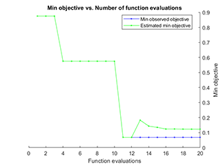
• Parameter Optimization using Bayesian optimization, Genetic Algorithm, and Particle Swarm Optimization
• Weighted SVDD model

Notices

• This version of the code is not compatible with the versions lower than R2016b.
• The label must be 1 for positive sample or -1 for negative sample.
• Detailed applications please see the demonstrations.
• This code is for reference only.

How to use

01. banana-shaped dataset

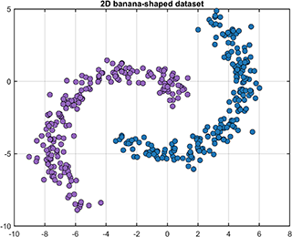
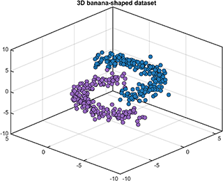
A class named DataSet is defined to generate and partition the 2D or 3D banana-shaped dataset.

[data, label] = DataSet.generate;
[data, label] = DataSet.generate('dim', 2);
[data, label] = DataSet.generate('dim', 2, 'num', [200, 200]);
[data, label] = DataSet.generate('dim', 3, 'num', [200, 200], 'display', 'on');

% 'single' --- The training set contains only positive samples. 
[trainData, trainLabel, testData, testLabel] = DataSet.partition(data, label, 'type', 'single');

% 'hybrid' --- The training set contains positive and negetive samples. 
[trainData, trainLabel, testData, testLabel] = DataSet.partition(data, label, 'type', 'hybrid');

02. Kernel funcions

A class named Kernel is defined to compute kernel function matrix.

%{
        type   -
        
        linear      :  k(x,y) = x'*y
        polynomial  :  k(x,y) = (γ*x'*y+c)^d
        gaussian    :  k(x,y) = exp(-γ*||x-y||^2)
        sigmoid     :  k(x,y) = tanh(γ*x'*y+c)
        laplacian   :  k(x,y) = exp(-γ*||x-y||)
    
    
        degree -  d
        offset -  c
        gamma  -  γ
%}
kernel = Kernel('type', 'gaussian', 'gamma', value);
kernel = Kernel('type', 'polynomial', 'degree', value);
kernel = Kernel('type', 'linear');
kernel = Kernel('type', 'sigmoid', 'gamma', value);
kernel = Kernel('type', 'laplacian', 'gamma', value);

For example, compute the kernel matrix between X and Y

X = rand(5, 2);
Y = rand(3, 2);
kernel = Kernel('type', 'gaussian', 'gamma', 2);
kernelMatrix = kernel.computeMatrix(X, Y);
>> kernelMatrix

kernelMatrix =

    0.5684    0.5607    0.4007
    0.4651    0.8383    0.5091
    0.8392    0.7116    0.9834
    0.4731    0.8816    0.8052
    0.5034    0.9807    0.7274

03-1. Simple SVDD model for dataset containing only positive samples

[data, label] = DataSet.generate('dim', 3, 'num', [200, 200], 'display', 'on');
[trainData, trainLabel, testData, testLabel] = DataSet.partition(data, label, 'type', 'single');
kernel = Kernel('type', 'gaussian', 'gamma', 0.2);
cost = 0.3;
svddParameter = struct('cost', cost,...
                       'kernelFunc', kernel);
svdd = BaseSVDD(svddParameter);

% train SVDD model
svdd.train(trainData, trainLabel);
% test SVDD model
results = svdd.test(testData, testLabel);

In this code, the input of svdd.train is also supported as:

% train SVDD model
svdd.train(trainData);

The training and test results:

*** SVDD model training finished ***
running time            = 0.0069 seconds
iterations              = 9 
number of samples       = 140 
number of SVs           = 23 
radio of SVs            = 16.4286% 
accuracy                = 95.0000%


*** SVDD model test finished ***
running time            = 0.0013 seconds
number of samples       = 260 
number of alarm points  = 215 
accuracy                = 94.2308%

03-2. Simple SVDD model for dataset containing both positive and negetive samples

[data, label] = DataSet.generate('dim', 3, 'num', [200, 200], 'display', 'on');
[trainData, trainLabel, testData, testLabel] = DataSet.partition(data, label, 'type', 'hybrid');
kernel = Kernel('type', 'gaussian', 'gamma', 0.05);
cost = 0.9;
svddParameter = struct('cost', cost,...
                       'kernelFunc', kernel);
svdd = BaseSVDD(svddParameter);

% train SVDD model
svdd.train(trainData, trainLabel);
% test SVDD model
results = svdd.test(testData, testLabel);

The training and test results:

*** SVDD model training finished ***
running time            = 0.0074 seconds
iterations              = 9 
number of samples       = 160 
number of SVs           = 12 
radio of SVs            = 7.5000% 
accuracy                = 97.5000%


*** SVDD model test finished ***
running time            = 0.0013 seconds
number of samples       = 240 
number of alarm points  = 188 
accuracy                = 96.6667%

04. Visualization

A class named SvddVisualization is defined to visualize the training and test results.

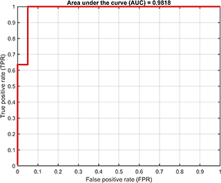
Based on the trained SVDD model, the ROC curve of the training results (only supported for dataset containing both positive and negetive samples) is

% Visualization 
svplot = SvddVisualization();
svplot.ROC(svdd);

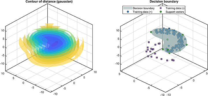
The decision boundaries (only supported for 2D/3D dataset) are

% Visualization 
svplot = SvddVisualization();
svplot.boundary(svdd);

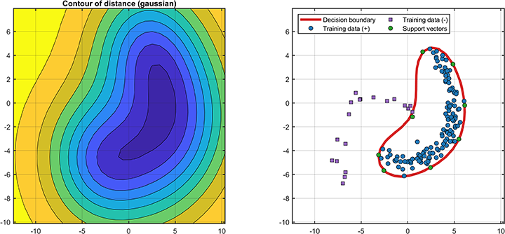
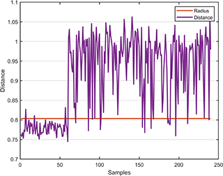
The distance between the test data and the hypersphere is

svplot.distance(svdd, results);

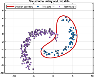
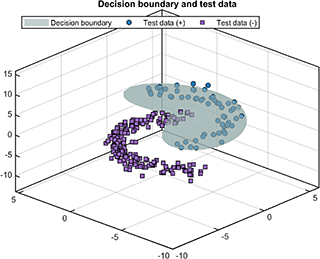
For the test results, the test data and decision boundary (only supported for 2D/3D dataset) are

svplot.testDataWithBoundary(svdd, results);

05. Parameter Optimization

A class named SvddOptimization is defined to optimized the parameters.

% optimization setting 
optimization.method = 'bayes'; % bayes, ga  pso 
optimization.variableName = { 'cost', 'gamma'};
optimization.variableType = {'real', 'real'}; % 'integer' 'real'
optimization.lowerBound = [10^-2, 2^-6];
optimization.upperBound = [10^0, 2^6];
optimization.maxIteration = 20;
optimization.points = 10;
optimization.display = 'on';

% SVDD parameter
svddParameter = struct('cost', cost,...
                       'kernelFunc', kernel,...
                       'optimization', optimization);

The visualization of parameter optimization is

Notice

• The optimization method can be set to 'bayes', 'ga', 'pso'.
• The parameter names are limited to 'cost', 'degree', 'offset', 'gamma'
• The parameter optimization of the polynomial kernel function can only be achieved by using Bayesian optimization.
• The parameter type of 'degree' should be set to 'integer'.

06. Cross Validation

In this code, two cross-validation methods are supported: 'K-Folds' and 'Holdout'. For example, the cross-validation of 5-Folds is

svddParameter = struct('cost', cost,...
                       'kernelFunc', kernel,...
                       'KFold', 5);

For example, the cross-validation of the Holdout method with a ratio of 0.3 is

svddParameter = struct('cost', cost,...
                       'kernelFunc', kernel,...
                       'Holdout', 0.3);

07. Dimensionality reduction using PCA

For example, reducing the data to 2 dimensions can be set as

% SVDD parameter
svddParameter = struct('cost', cost,...
                       'kernelFunc', kernel,...
                       'PCA', 2);

Notice: you only need to set PCA in svddParameter, and you don't need to process training data and test data separately.

08. Weighted SVDD

An Observation-weighted SVDD is supported in this code. For example, the weighted SVDD can be set as

weight = rand(size(trainData, 1), 1);
% SVDD parameter
svddParameter = struct('cost', cost,...
                       'kernelFunc', kernel,...
                       'weight', weight);

Notice: the size of 'weigh' should be m×1， where m is the number of training samples.