GAN_PyTorch

Various GAN implementations based on PyTorch. This project is consist of simple and standard version. The Simple version has a relatively short code length, and only simple functions are implemented.
The Standard version has various functions rather than the simple version. It also provides a UI using PyQt(In this case, the standard version is loaded and executed). In fact, I don't know if UI is comfortable...

Implementation list

• Vanilla GAN : Simple | Standard & UI
• DCGAN : Simple |
• InfoGAN : Simple |

Experiment Environment

• Windows 10 Enterprise
• Intel i7-3770k
• RAM 12.0 GB
• NVIIDA GTX TITAN
• Python 3.6.4
• PyTorch 0.4.0
• torchvision 0.2.1
• PyQt 5
• CUDA 9.0
• cuDNN 7.1.4

1. Vanilla_GAN

MLP-based regular GAN is implemented. Ian Goodfellow's paper used Maxout, ReLU, and SGD. But the performance is not working properly, so I modified it and implemented it.
Paper

1.1 Vanilla_Simple.py

• This is a brief implementation of the Vanilla GAN, and the functions are described below by block.
• This code refers to the following code.

• This code uses the MNIST data set.

1) Import

Import the necessary libraries.

• torch : Library to implement tensor or network structures
• torchvision : Library for managing datasets
• os : Library for loading file path

import torch as tc
import torch.nn as nn
import torchvision
import torchvision.transforms as transforms
from torchvision.utils import save_image
import os

2) Parameter

Set the image size, result path, and hyper parameter for learning.

• result_path : Path where the results are saved.
• img_sz : Image size.(MNIST =28)
• noise_sz : Latent code size which is the input of generator.
• hidden_sz : Hidden layer size.(The number of nodes per hidden layer)
• batch_sz : Batch size.
• nEpoch : Epoch number.
• nChannel : Channel size.(MNIST=1)
• lr : Learning rate.

result_path = 'simple'
img_sz = 784
noise_sz = 100
hidden_sz = 512
batch_sz = 100
nEpoch = 300
nChannel = 1
lr = 0.0002

3) Data load

Load the dataset. This project used MNIST dataset.

• trans : Transform the dataset.

  • Compose()is used when there are multiple transform options. Here, ToTensor() and Normalize(mean, std) are used.
  • ToTensor () changes the PIL Image to a tensor. torchvision dataset The default type is PIL Image.
  • Normalize (mean, std) transforms the range of the image. Here, the value of [0, 1] is adjusted to [-1, 1]. ((value-mean) / std)

• dataset : Load (MNIST data) at the specified location.

  • root : This is the path to store (MNIST data). Folders are automatically created with the specified name.
  • train : Set the data to be used for the train.
  • transform : Transform the data according to the transform option set previously.
  • download : Download (MINST data). (If you downloaded it once, it will not do it again.)

• dataloader : Load the data in the dataset.

  • dataset : Set the dataset to load.
  • batch_size : Set the batch size.
  • shuffle : Shuffle the data and load it.

trans = transforms.Compose([transforms.ToTensor(), transforms.Normalize((0.5, 0.5, 0.5), (0.5, 0.5, 0.5))])
dataset = torchvision.datasets.MNIST(root='./MNIST_data', train=True, transform=trans, download=True)
dataloader = tc.utils.data.DataLoader(dataset=dataset, batch_size=batch_sz, shuffle=True)

4) Range

[0, 1] in the range of [-1, 1].

• Clamp changes the value of 0 or less to 0, and the value of 1 or more to 1.

def img_range(x):
    out = (x+1)/2
    out = out.clamp(0, 1)
    return(out)

5) Discriminator

Create a Discriminator

• Sigmoid was placed on the last layer to output [0, 1]. (0 : Fake, 1 : Real)

D = nn.Sequential(
    nn.Linear(img_sz, hidden_sz),
    nn.ReLU(),
    nn.Linear(hidden_sz, hidden_sz),
    nn.ReLU(),
    nn.Linear(hidden_sz, 1),
    nn.Sigmoid()
)

6) Generator

Create a Generator

• Tanh is placed on the last layer to output [-1, 1].

G = nn.Sequential(
    nn.Linear(noise_sz, hidden_sz),
    nn.ReLU(),
    nn.Linear(hidden_sz, hidden_sz),
    nn.ReLU(),
    nn.Linear(hidden_sz, img_sz),
    nn.Tanh()
)

7) GPU

Pass the network to the GPU.

• If is_available () is true, the GPU is used. If it is false, CPU is used.

device = tc.device('cuda' if tc.cuda.is_available() else 'cpu')
D = D.to(device)
G = G.to(device)

8) Optimizer

Set the optimizer to optimize the loss function.

• Loss function is set to BCELoss () and Binary Cross Entropy Loss. The definition of BCE is BCE (x, y) = -y * log (x) - (1-y) * log (1-x).

loss_func = tc.nn.BCELoss()
d_opt = tc.optim.Adam(D.parameters(), lr=lr)
g_opt = tc.optim.Adam(G.parameters(), lr=lr)

9) Training

The training process consists of learning the discriminator and learning the generator.

9-1) Train the D

• Load the images from the dataloader
  
• Flatten the images in one dimension to fit MLP.
  
• Generate noise (lantic code) for the input of the generator.
  
• Create a label for discriminator learning.
  
• In Discriminator, Input the images and the fake images (G (z)). Find the loss function using labels (real: 1, fake: 0).
  
• Add each loss to find the total loss, and use the backward () function to find the gradient of each node. step () updates the parameters(w,b) according to the optimizer option defined above. Note that only the discriminator is learned.
  

for ep in range(nEpoch):
    for step, (images, _) in enumerate(dataloader):
        images = images.reshape(batch_sz, -1).to(device)
        z = tc.randn(batch_sz, noise_sz).to(device)

        real_label = tc.ones(batch_sz, 1).to(device)
        fake_label = tc.zeros(batch_sz, 1).to(device)

        loss_real = loss_func(D(images), real_label)
        loss_fake = loss_func(D(G(z)), fake_label)

        d_loss = loss_real + loss_fake

        d_opt.zero_grad()
        d_loss.backward()
        d_opt.step()

9-2) Train the G

• Perform the learning in a similar way as before. Note that only learn about the generator.
  

        fake_images = G(z)
        g_loss = loss_func(D(fake_images), real_label)

        g_opt.zero_grad()
        g_loss.backward()
        g_opt.step()

10) Log and Image save

Print the log and seve the image.

        if step%200 ==0:
            print('epoch {}/{}, step {}, d_loss {:.4f}, g_loss {:.4f}, Real_score {:.2f}, Fake_score {:.2f}'.format(ep, nEpoch, step+1, d_loss.item(), g_loss.item(), D(images).mean().item(), D(fake_images).mean().item()))

    if ep==0:
        out = images.reshape(mini, nChannel, img_sz, img_sz)
        out = img_range(out)
        save_image(out, os.path.join(result_path, 'real_img.png'))
    out = fake_images.reshape(mini, nChannel, img_sz, img_sz)
    out = img_range(out)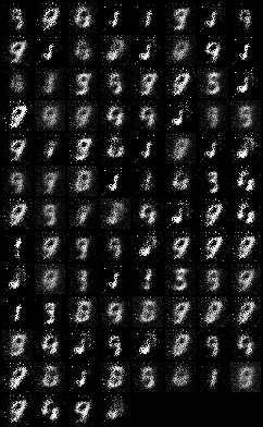
    save_image(out, os.path.join(result_path, 'fake_img {}.png'.format(ep)))

11) Results

The figure below shows the results as the epoch increases.(1, 15, 60, 1000)

1.2 Vanilla_Standard.py and for_UI.py

• The UI supports batch size, epoch size, learning rate, and dataset settings.
• Save the log file as csv.
  

2. DCGAN

Deep Convolutional GAN is implemented.
Paper

2.1 DCGAN_Simple.py

• This is a brief implementation of the DCGAN. This code uses CelebA dataset.
• LSUN is available here.
  • Run download.py to download the LSUN data.
  • If you are using Python 3.0 or later, modify the code from urllib2.urlopen (url) to urlopen (url).

  def list_categories(tag):
    url = 'http://lsun.cs.princeton.edu/htbin/list.cgi?tag=' + tag
    f = urlopen(url)
    return json.loads(f.read())
• This code refers to the following code1 and code2.

1) Data load

Load the dataset. This project used CelebA dataset.

• trans : Transform the dataset.

  • Compose()is used when there are multiple transform options. Here, Resize(), ToTensor() and Normalize(mean, std) are used.
  • Resize() is used to resize the image.
  • ToTensor () changes the PIL Image to a tensor. torchvision dataset The default type is PIL Image.
  • Normalize (mean, std) transforms the range of the image. Here, the value of [0, 1] is adjusted to [-1, 1]. ((value-mean) / std)

• dataset : Load (CelebA data) at the specified location.

  • ImageFolder(path, trans) : The data in the path is loaded according to the trans option.
  • If you want to use LSUN, change from ImageFolder('./img_align_celeba', trans) to LSUN('.', classes=['bedroom_train'], transform=trans).
  • The data must be in the same path.

• dataloader : Load the data in the dataset.

  • dataset : Set the dataset to load.
  • batch_size : Set the batch size.
  • shuffle : Shuffle the data and load it.

trans = transforms.Compose([transforms.Resize((img_sz, img_sz)), transforms.ToTensor(), transforms.Normalize((0.5, 0.5, 0.5), (0.5, 0.5, 0.5))])
dataset = tv.datasets.ImageFolder('./img_align_celeba', trans)
dataloader = tc.utils.data.DataLoader(dataset=dataset, batch_size= batch_sz, shuffle= True)

2) Generator

Create a Generator

• Used 5 transposed convolutional layers and 4 batch normalizations. Tanh is placed on the last layer to output [-1, 1].

class Generator(nn.Module):
    def __init__(self, latent_sz):
        super(Generator, self).__init__()
        self.tconv1 = nn.ConvTranspose2d(latent_sz, 1024, 4, 1, 0)
        self.tconv2 = nn.ConvTranspose2d(1024, 512, 4, 2, 1)
        self.tconv3 = nn.ConvTranspose2d(512, 256, 4, 2, 1)
        self.tconv4 = nn.ConvTranspose2d(256, 128, 4, 2, 1)
        self.tconv5 = nn.ConvTranspose2d(128, 3, 4, 2, 1)

        self.bn1 = nn.BatchNorm2d(1024)
        self.bn2 = nn.BatchNorm2d(512)
        self.bn3 = nn.BatchNorm2d(256)
        self.bn4 = nn.BatchNorm2d(128)

    def forward(self, input):
        x = F.relu(self.bn1(self.tconv1(input)))
        x = F.relu(self.bn2(self.tconv2(x)))
        x = F.relu(self.bn3(self.tconv3(x)))
        x = F.relu(self.bn4(self.tconv4(x)))
        x = F.tanh(self.tconv5(x))

        return x

    def weight_init(self, mean, std):
        for m in self._modules:
            normal_init(self._modules[m], mean, std)

3) Discriminator

Create a Discriminator

• Used 5 convolutional layers and 3 batch normalizations. Sigmoid was placed on the last layer to output [0, 1].

class Discriminator(nn.Module):
    def __init__(self):
        super(Discriminator, self).__init__()
        self.conv1 = nn.Conv2d(3, 128, 4, 2, 1)
        self.conv2 = nn.Conv2d(128, 256, 4, 2, 1)
        self.conv3 = nn.Conv2d(256, 512, 4, 2, 1)
        self.conv4 = nn.Conv2d(512, 1024, 4, 2, 1)
        self.conv5 = nn.Conv2d(1024, 1, 4, 1, 0)

        self.bn2 = nn.BatchNorm2d(256)
        self.bn3 = nn.BatchNorm2d(512)
        self.bn4 = nn.BatchNorm2d(1024)

    def forward(self, input):
        x = F.leaky_relu(self.conv1(input), 0.2)
        x = F.leaky_relu(self.bn2(self.conv2(x)), 0.2)
        x = F.leaky_relu(self.bn3(self.conv3(x)), 0.2)
        x = F.leaky_relu(self.bn4(self.conv4(x)), 0.2)
        x = F.sigmoid(self.conv5(x))

        return x

    def weight_init(self, mean, std):
        for m in self._modules:
            normal_init(self._modules[m], mean, std)

4) Weight & Bias initialization

The weights of nn.ConvTransposed2d or nn.Conv2d are initialized by normal distribution. Their biases are initialized to zero.

def normal_init(m, mean, std):
    if isinstance(m, nn.ConvTranspose2d) or isinstance(m, nn.Conv2d):
        m.weight.data.normal_(mean, std)
        m.bias.data.zero_()

5) Other functions

It is very similar to the vanilla gan described above.

6) Results

The figure below shows the results as the epoch increases.

6-1) CelebA

• real
  
• epoch 1
  
• epcoh 5
  
• epoch 30
  

6-2) LSUN

• real
  
• epoch 1
  
• epoch 2
  
• epoch 5
  

6-3) Koeran Idol(Black Pink)

Data can be downloaded here.

• real
  
• epoch 1
  
• epoch 5
  
• epoch 100
  
• epoch 150
  

3. InfoGAN

Information Maximizing GAN is implemented. It is implemented based on DCGAN.(Not MLP)
Paper

3.1 InfoGAN_Simple.py

• This is a brief implementation of the InfoGAN. This code uses MNIST dataset.
• If you want to use LSUN and CelebA, see here.
• If you want to use 3d chair dataset, you can download it here.
• This code refers to the following code.

1) Data load

Load the dataset. This project used MNIST dataset.

• trans : Transform the dataset.

  • Compose()is used when there are multiple transform options. Herem ToTensor() and Normalize(mean, std) are used.
  • Resize() is used to resize the image.
  • ToTensor () changes the PIL Image to a tensor. torchvision dataset The default type is PIL Image.
  • Normalize (mean, std) transforms the range of the image. Here, the value of [0, 1] is adjusted to [-1, 1]. ((value-mean) / std)

• dataset : Load (MNIST data) at the specified location.

  • ImageFolder(path, trans) : The data in the path is loaded according to the trans option.
  • If you want to use LSUN, change from ImageFolder('./img_align_celeba', trans) to LSUN('.', classes=['bedroom_train'], transform=trans).
  • The data must be in the same path.

• dataloader : Load the data in the dataset.

  • dataset : Set the dataset to load.
  • batch_size : Set the batch size.
  • shuffle : Shuffle the data and load it.

will be updated

2) Generator

Create a Generator

• Used 5 transposed convolutional layers and 4 batch normalizations. Tanh is placed on the last layer to output [-1, 1].

will be updated

3) Discriminator

Create a Discriminator

• Used 5 convolutional layers and 3 batch normalizations. Sigmoid was placed on the last layer to output [0, 1].

will be updated

4) Latent Code and Loss

Create latent codes(noise, dc, cc) and compute the loss.

will be updated

5) Other functions

It is very similar to the vanilla gan described above.

6) Results

The figure below shows the results according to dc(discrete code, categorical code) and cc(continous code).

6-1) MNIST

• result
  will be updated

6-2) CelebA

• result
  will be updated

6-3) 3D Chair

• result
  will be updated