Our tutorial is only lasting a few hours and because we don't have a significant amount of resources to use, we will be using a subset WGBS sequencing run as today's dataset. To further reduce the strains on our resources, we'll be mapping our dataset against the model plant genome Arabidopsis_thaliana, which co-incidently was one of the first organisms to be run using whole-genome bisulfite sequencing (WGBS/BS-seq/MethylC-seq) in Ryan Lister's 2008 Cell paper. Arabidopsis_thaliana is roughly 125Mb in size, making it a easy organism to map to, and there have been some great papers published which sequence the methylomes of a range of DNA methyltransferase (DNMT) mutants.
In this tutorial we're taking two samples from the paper:
Stroud H, Greenberg MV, Feng S, Bernatavichute YV, Jacobsen SE. Comprehensive analysis of silencing mutants reveals complex regulation of the Arabidopsis methylome. Cell. 2013 Jan 17;152(1-2):352-64. doi: 10.1016/j.cell.2012.10.054. Epub 2013 Jan 11. Erratum in: Cell. 2015 Jun 18;161(7):1697-8. PMID: 23313553; PMCID: PMC3597350.

For plant researchers, or anyone interested in the mechanisms of DNA methylation maintenance for that matter, this paper is a great resource. There is a significant amount of sequencing data produced from Arabidopsis thaliana lines that contain silencing mutations in genes involved in DNA methylation-derived gene regulation. All these sequencing datasets are publicly available and can be used to study how methyltransferases deposit DNA methylation markers and what genes are regulated by each. Most of these mutants have multiple replicates, but for today we are going to be taking a subset of two WGBS libraries sequenced from a cytosine-DNA-methyltransferase gene mutant (met1) and the standard Col or Columbia ecotype (colWT). MET1 is the gene responsible for the maintenance of CpG methylation in Plants, so silencing this gene has a major impact on DNA methylation throught the organism.
The FASTQ files that are needed for today's tutorial are in the /data/wgbs/ and named SRR534177_colWT.fastq.gz and SRR534239_met1.fastq.gz.
We need to copy the data into our home directory by running:
# copy everything from /data/wgbs to our home dir
cp /data/wgbs/* ~/
These FASTQs are a subset of reads (~6M) that map to chr1 and chloroplast chromosomes of Arabidopsis thaliana in order to speed up analysis time.
Lets have a look at these FASTQs by using the zcat and head linux functions which allow us to print out a compressed file (i.e. SRR534239_met1.fastq.gz) and only take the top or head of the file.
These two commands are executed together with the help of the pipe (|) function, which reads the output of the first command (zcat) and uses that as the input for the second command (head -n 8).
Here we only take the first 8 lines (first 2 reads of each sample) with the command head -n 8.
$ zcat SRR534239_met1.fastq.gz | head -n 8
@SRR534239.8 SN971_XB024:1:1101:47.20:97.70/1
NTAAATGGAAAATGATATTGAGAGTATTTTGGAGTTTTAGAGTATATTGG
+
!1:DDFFFHHHHHJJJJJJJIIEHC,AHIIJJCGEGIJGIHICFHIJJJJ
@SRR534239.12 SN971_XB024:1:1101:67.80:95.30/1
NATTAGGTATGGAATTTTAAATAGAATAGAGAATGTTGAATTAGATTGAG
+
!1=DDFFDHHHHHJJJJJJJJJJIJJJIIHIGIJJJJJIJJJJJJJJJJJ


$ zcat SRR534177_colWT.fastq.gz | head -n 8
@SRR534177.13 SN603_WA034:3:1101:45.50:110.90/1
ATTTTATTTTATAAAATTTTATTATATGTATGTGAATATGCGATTATTTG
+
@@@ADDDDHFFBFBHIIIIGIIIAHBEEFFHBBHBHCBH>4?EHGIGIIG
@SRR534177.18 SN603_WA034:3:1101:42.80:117.20/1
GAAAGGGTACGGATTTAACAAAATAATGGTATAATTTTTAGAGTAGTACC
+
@@@FFDF?DFHHFGGHGGBHGGIFGGEGG9?FGIIJJJJIIIIBFHHHIJ
As you see, there's a lot of information in these files, much of which we will not be going into today. If you would like more detail on FASTQ format, see this excellent explaination at the University of Adelaide Bioinformatics Hub's "Intro to NGS" tutorial.
Questions
- What type of sequencing was carried out for these samples? Paired or single end sequencing?
- What was the read-length of the sequencing run?
The important first step in any pipeline is assessing the quality of your initial dataset. Just because a dataset has been published, does not mean that its of high quality (quite the opposite in our experience!). For most of our pipelines and workflows, we run a standard FastQC analysis.
# Run fastQC
fastqc -t 2 SRR534239_met1.fastq.gz SRR534177_colWT.fastq.gz
This command creates a nice little HTML report for us to view, however we'll need to transfer it back to our local computers to view. NOTE: This command MUST be run from your local machine, not the VM, and that you'll need to change the name of the file location and username/host address to fit your situation.
# Move the FastQC report from the VM to your home
scp jimmy.breen@myhost.com.au:*_fastqc.html ~/tutorial/
Please let a helper know if you're having issues. Example HTML files are available below, but you will need to download these to your computer to view.
- https://github.com/sagc-bioinformatics/SAGC_5mCMethylation_tutorial/blob/7d7fbd0eb8c3b5fa17a01e6cb68d6a9158f2dc2a/data/SRR534177_colWT_fastqc.html
- https://github.com/sagc-bioinformatics/SAGC_5mCMethylation_tutorial/blob/7d7fbd0eb8c3b5fa17a01e6cb68d6a9158f2dc2a/data/SRR534239_met1_fastqc.html
Questions
- How many total reads are in each sample?
- How do the "Per base sequence content" graphs of both samples compare?
- How much adapter contamination do we see in each sample?
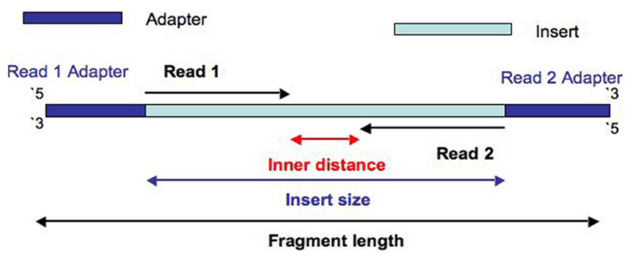
Similar to other forms of high-throughput sequencing data, adapter contamination and/or poor sequence quality has the ability to impact downstream genome mapping procedures. Adapter contamination for example, is a common issue with WGBS protocols, as the Sodium bisulfite (NaHSO3) treatment can damage and fragment DNA reducing the fragment/insert size. A smaller insert size that the sequencing read length then leads to adapters being present in the sequencing data.
While we don't see a massive amount of adapter contamination on our FastQC report, lets
We may need to trim quality and adapters if the fastQC report indicates that there is adapter contamination and/or poor quality at the end of sequence reads.
# SRR534239 trimming
trim_galore -o ./ --clip_R1 5 --three_prime_clip_R1 5  SRR534177_colWT.fastq.gz

# SRR534239 trimming
trim_galore -o ./ --clip_R1 5 --three_prime_clip_R1 5  SRR534239_met1.fastq.gz
As you can see here, there are a two parameters --clip_R1 5 --three_prime_clip_R1 5 that are added to the trimming command for each sample.
The trimming of bases at either end of the fragment is a relatively standard procedure in WGBS data. This is mainly driven by random priming oligos that are used to amplify bisulfite converted DNA at the library preparation stage.
See this data processing section from a recent Systematic Evaluation of WGBS library preparation methods (Zhou et al. 2019 Scientific Reports):
"Raw sequencing output BCL data were converted to FASTQ files by using bcl2fastq v2.20 software53. The sequence quality was checked by FastQC v0.11.554. Adaptors and low quality sequences (Phred <20) were trimmed by Trim Galore v0.4.4_dev and cutadapt v1.1555,56. Different additional trimming were applied according to the library preparation method used. As random oligos (6N) and low complexity tail (8N) introduced during TruSeq and Swift library preparation respectively would lead to artifactual cytosine methylation calling and low quality sequencing bases, nucleotide trimming is recommended. We tested parameters with different levels of stringency to optimize the trimming criteria in an effort to strike a balance between mapping rates and depth of coverage. For the QIAseq method, although no length information of the oligos used for random priming was provided from the library preparation protocol, we similary tested different parameters at varying strigency and arrived at the current parameters which balances amount of data loss (coverage depth) and mapping efficiency. The final trimming parameters were as follows: Swift:–clip_R2 18–three_prime_clip_R1 18; TruSeq:–clip_R1 8–clip_R2 8–three_prime_clip_R1 8–three_prime_clip_R2 8; QIAseq:–clip_R1 10–clip_R2 10. Trimmed reads were checked by FastQC again before mapping to bisulfite-converted hg19 genome by bismark30."_

Library preparation methods differ, so always check your data quality report first and the data analysis documentation for the specific WGBS kit you are using.
Let's have a look at the final trimming results to see how much we've actually trimmed?
$ ls -1 SRR534177_colWT*
SRR534177_colWT_fastqc.html
SRR534177_colWT_fastqc.zip
SRR534177_colWT.fastq.gz
SRR534177_colWT.fastq.gz_trimming_report.txt
SRR534177_colWT_trimmed.fq.gz
The trim-galore report is contained within the file finishing with the suffix _trimming_report.txt, so lets have a look at it.
$ less SRR534177_colWT.fastq.gz_trimming_report.txt
Questions
- What type of adapter was detected and used in the
trim-galoretrimming? - What proportion of reads had adapters in each sample?
- How many sequences in each sample were removed due to being smaller than the 20bp minimum sequence?
Its a question we get a lot: "So how much coverage do I need?" Well as with all questions you get with high-throughput sequencing, it depends on the question you want answered. Based on our experience, specific levels of coverage impact specific biological questions.
Below is a basic guide to identify the right coverage for the right analysis:
Low coverage (1-10X genome coverage):
- Good for identifying global DNA methylation patterns and comparing samples
- Good for identifying large regions of DNA methylation change
- Will not give methylation signal for every cytosine
- Limits the accuracy of DMR detection
High coverage (30X+ genome coverage):
- Close to single C coverage
- Accurate DMRs and methylation signal at each site
- Potentially identify haplotype-specific DNA methylation (may require 50X+ coverage)
With Differentially Methylated Region (DMR) identification, you should be looking at a minimum of 3 replicates per group for species with low genetic variability (i.e. model organisms). For humans and other species that lack extensive inbreeding, you should be aiming for 4+ replicates.
NEXT: We'll dive into Genome Mapping