bayoudev
This tutorial guides the user through using some of the development features of bayou, including a new method of running mcmc objects and loading the data back into R, as well as increased capacity for including predictor variables. This is in constant development, so please bear with me as I increase functionality and options.
In this example, we will use bayou chelonia dataset to simulate data and estimate the simulated relationships. First, we need to install the development version of bayou.
require(devtools)
require(geiger)
install_github('uyedaj/bayou', ref = 'dev')
## Downloading github repo uyedaj/bayou@dev
## Installing bayou
## '/usr/lib/R/bin/R' --vanilla CMD INSTALL \
## '/tmp/RtmpZjl13c/devtools4fe078fddc37/uyedaj-bayou-dfe12a4' \
## --library='/home/josef/R/x86_64-pc-linux-gnu-library/3.1' \
## --install-tests
##
## Reloading installed bayou
require(bayou)Now we need to simulate allometric relationships.
data(chelonia)
tree <- chelonia$phy
ntips <- length(chelonia$phy$tip.label)
pred <- cbind(chelonia$dat)
true.pars <- list(alpha=1, sig2=1, beta1=0.75, k=3, ntheta=4, theta=c(2,3,1,8))
Now we need to set where the shifts occur on the tree. We can do this manually, or interactively using bayou's "identifyBranches" function. This function will require you to click on 'k' branches to assign regimes.
shifts <- identifyBranches(tree, true.pars$k)Now use the output to generate the simulated data. This will be more clean in the future, but for now this works.
true.pars$sb <- shifts$sb
true.pars$loc <- shifts$loc
true.pars$t2 <- 2:true.pars$ntheta
dat <- dataSim(true.pars, model = "OU", tree, SE=0)$dat
## [1] "Using mapped regimes from parameter list"
cache <- bayou:::.prepare.ou.univariate(tree, dat,SE=0, pred=pred)
nn <- names(dat)
dat <- dat + true.pars$beta1*cache$pred
dat <- dat[,1]
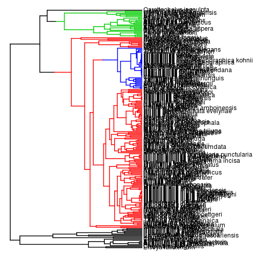
names(dat) <-nnLet's look at the simulated data. Shift locations:
tr <- pars2simmap(true.pars, tree)
plotSimmap(tr$tree, colors=tr$cols)
## no colors provided. using the following legend:
## 1 2 3 4
## "black" "red" "green3" "blue"
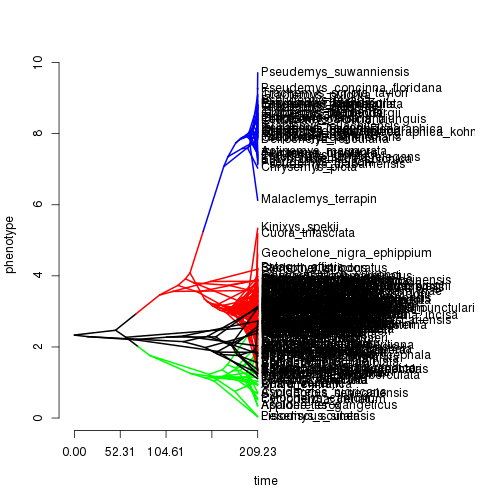
 Phenogram:
phenogram(tr$tree, dat, colors=tr$cols)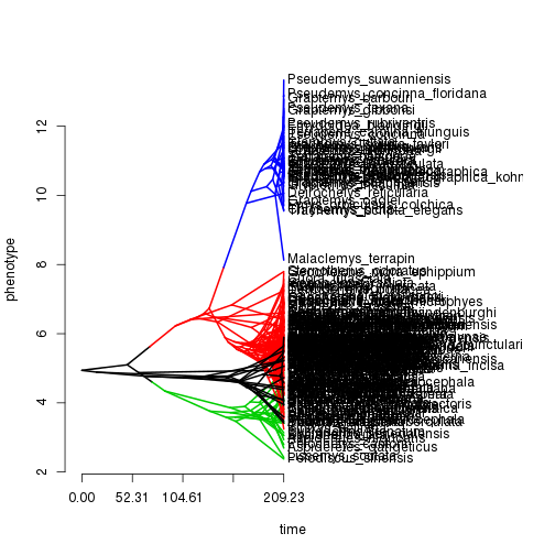 Scatterplot against predictor variables:
plot(cache$pred, dat)
Make the prior.
prior <- make.prior(tree, dists=list(dalpha="dhalfcauchy", dsig2="dhalfcauchy",
                                     dbeta1="dunif", dsb="dsb", dk="cdpois", dtheta="dunif"),
                      param=list(dalpha=list(scale=1), dsig2=list(scale=1),
                              dbeta1=list(min=-10, max=10), dk=list(lambda=15, kmax=200), dsb=list(bmax=1,prob=1),
                                    dtheta=list(min=0, max=15)), model="ffancova")
Make sure the prior function works:
prior(true.pars)## [1] -41.31
First step is to create the MCMC object that will run our MCMC chain.
mymcmc <- bayou.makeMCMC(tree, dat, pred, SE=0, model="ffancova", prior=prior, startpar=list(alpha=0.1, sig2=3, beta1=1, k=1, ntheta=2, theta=c(4,4), sb=200, loc=0, t2=2), new.dir=TRUE, ticker.freq=1000)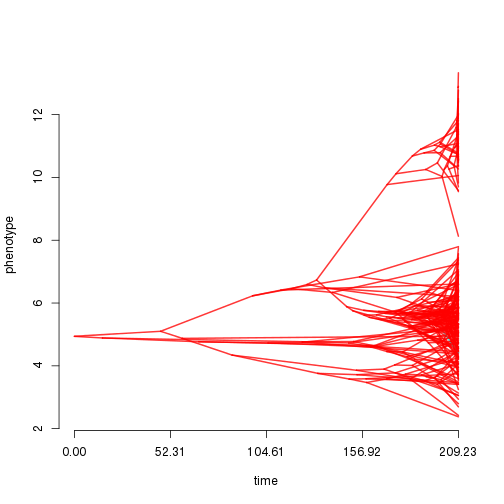
To execute the MCMC, specify the number of steps in parentheses. Additional calls using the same function will restart the chain where the previous run left off.
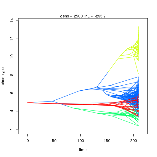
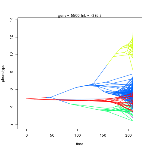
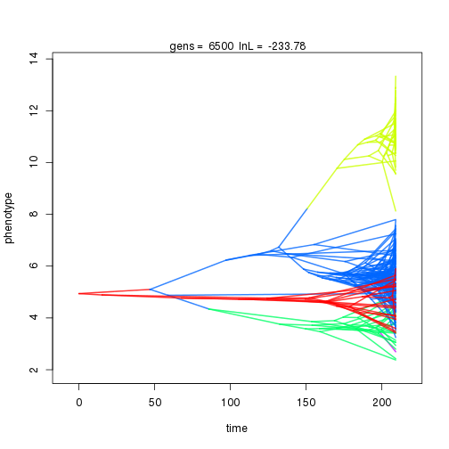
mymcmc$run(10000)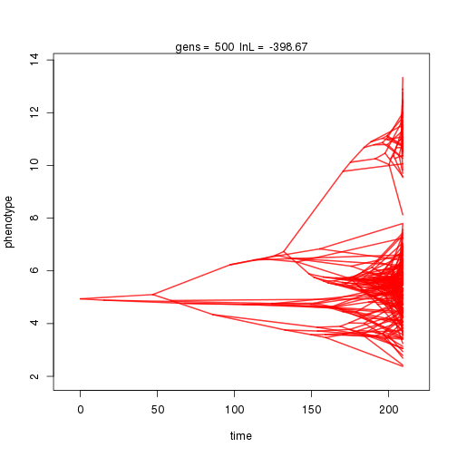
## gen     lnL     prior   alpha   beta1   sig2    k       .alpha  .beta1  birth.k D0.slid D1.slid death.k .sig2   .theta  U0.slid U1.slid U2.slid
## 1000    -240.12 -40.37  0.48    0.51    0.82    3       0.43    0.16    0.01    0.92    0.50    1.00    0.37    0.56    1.00    0.50    0.08
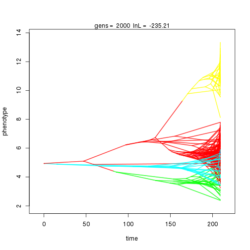
## 2000 -235.21 -54.01 1.29 1.21 0.90 5 0.36 0.13 0.01 0.94 0.42 0.45 1.00 0.34 0.44 1.00 0.40 0.11
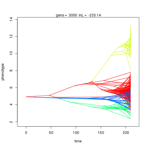
## 3000 -233.14 -47.39 1.05 0.92 0.96 4 0.32 0.11 0.01 0.84 0.38 0.50 0.75 0.32 0.41 1.00 0.33 0.09
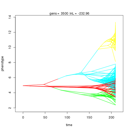

## 4000 -234.15 -53.11 0.82 0.76 0.91 5 0.32 0.09 0.01 0.86 0.38 0.53 0.67 0.30 0.42 1.00 0.32 0.10

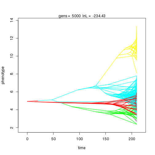
## 5000 -234.43 -53.10 0.79 0.79 0.96 5 0.32 0.09 0.01 0.87 0.39 0.46 0.57 0.31 0.41 1.00 0.36 0.09

## 6000 -231.57 -59.91 1.28 1.01 0.99 6 0.33 0.08 0.01 0.88 0.38 0.46 0.50 0.29 0.39 0.99 0.38 0.10
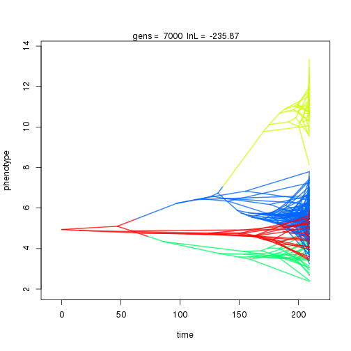
## 7000 -235.87 -47.39 0.94 1.04 0.97 4 0.33 0.08 0.01 0.89 0.39 0.42 0.50 0.30 0.37 0.99 0.35 0.10
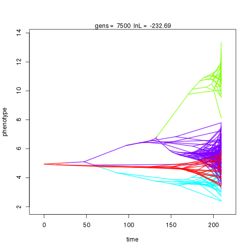
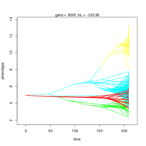
## 8000 -230.95 -52.92 0.71 0.67 0.99 5 0.33 0.07 0.01 0.90 0.41 0.42 0.44 0.30 0.34 0.99 0.33 0.09

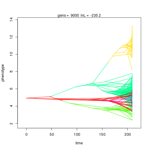
## 9000 -235.20 -61.70 2.35 1.98 1.04 6 0.34 0.07 0.01 0.90 0.41 0.43 0.44 0.30 0.34 0.99 0.34 0.09

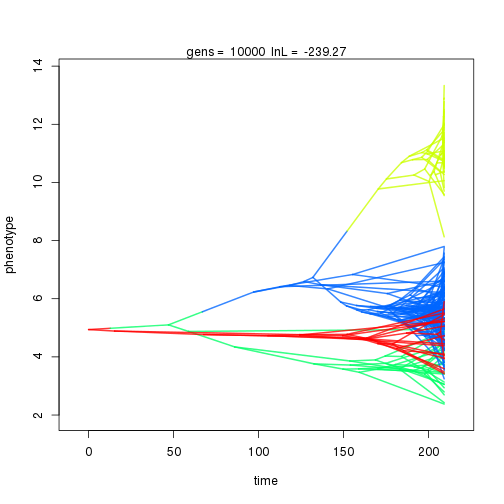
## 10000 -239.27 -47.39 0.91 1.06 1.02 4 0.34 0.06 0.01 0.91 0.44 0.43 0.44 0.30 0.35 0.99 0.35 0.09
Load the chain back into R using the '$load()' function.
chain <- mymcmc$load()Discard the initial burnin proportion
chain <- set.burnin(chain, 0.3)
sumchain <- summary(chain)
## bayou MCMC chain: 10000 generations
## 1001 samples, first 300 samples discarded as burnin
##
##
## Summary statistics for parameters:
## Mean SD Naive SE Time-series SE Effective Size
## lnL -234.5511 2.12238 0.080104 0.52245 16.503
## prior -51.8651 6.09419 0.230010 2.35806 6.679
## alpha 1.0310 0.30284 0.011430 0.09249 10.720
## sig2 0.9908 0.28482 0.010750 0.09595 8.811
## beta1 0.9798 0.03874 0.001462 0.01916 4.091
## k 4.7265 0.95959 0.036217 0.35216 7.425
## ntheta 5.7265 0.95959 0.036217 0.35216 7.425
## root.theta 1.3132 0.21949 0.008284 0.03086 50.597
## all theta 2.5152 2.42072 NA NA NA
##
##
## Branches with posterior probabilities higher than 0.1:
## pp magnitude.of.theta2 naive.SE.of.theta2 rel.location
## 400 1.0000 7.2201 0.007056 1.5643
## 49 0.9345 0.3964 0.007447 1.2234
## 411 0.5342 2.2601 0.006832 1.5949
## 450 0.4729 2.2165 0.019956 0.1402
## 16 0.3447 0.3708 0.035837 2.8876
## 340 0.1382 3.3443 0.027947 3.2317
## 249 0.1197 1.9894 0.041783 1.3707
## 266 0.1097 1.0044 0.053415 1.1746
## 269 0.1083 2.4467 0.076600 1.8459
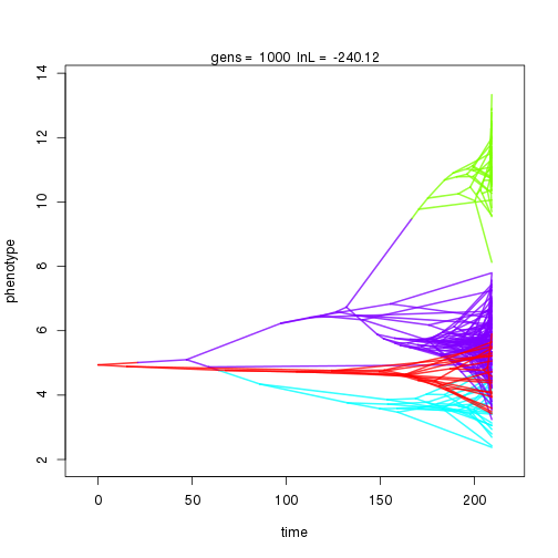
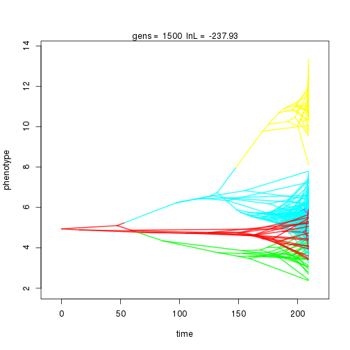
Plot showing the distributions of intercepts, note that if there are predictors this may be shifted away from the actual distribution of the data.
phenogram.density(tree, dat, chain=chain, burnin=0.3, pp.cutoff=0.3)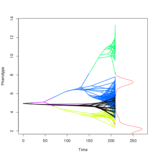 Check the chain for convergence.
plot(chain)

This is ugly code that I should have a function for, but it generates the median estimates of the parameters from the posterior distribution, as well as shift locations for all shifts that are in more than half of the posterior samples.
postburn <- round((0.3*length(chain$gen)),0):length(chain$gen)
est.pars <- list(alpha=median(chain$alpha[postburn]), sig2=median(chain$sig2[postburn]), beta1=median(chain$beta1[postburn]))
est.pars$sb <- which(sumchain$branch.posteriors[,1] > 0.5)
est.pars$k <- length(est.pars$sb)
est.pars$ntheta <- est.pars$k+1
est.pars$loc <- sumchain$branch.posteriors[est.pars$sb,4]
est.pars$t2 <- 1:length(est.pars$sb)+1
est.pars$theta <- c(median(sapply(chain$theta[postburn], function(x) x[1])), sumchain$branch.posteriors[est.pars$sb,2])
Generate a simmap tree from this median posterior estimate
tr <- pars2simmap(est.pars, tree)More code that to categorize the data based on which group they are found in in the posterior estimate.
tip.reg <- as.numeric(sapply(tr$tree$map, function(x) names(x)[length(x)]))
tip.reg <- tip.reg[which(tr$tree$edge[,2] <= ntips)]
o <- order(tr$tree$edge[,2][which(tr$tree$edge[,2] <= ntips)])
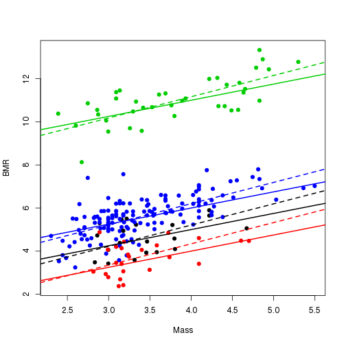
tip.reg <- tip.reg[o]Plotting routine to plot a scatter plot with the estimated and true regressions for the identified groups.
cache <- bayou:::.prepare.ou.univariate(tree, dat, SE=0, pred=pred)
plot(cache$pred, cache$dat, pch=21, bg=tip.reg, col=tip.reg, xlab="Mass", ylab="BMR")
for(i in 1:est.pars$ntheta){
  abline(a = est.pars$theta[i], b=est.pars$beta1, lwd=2, col=i,lty=2)
  on <- match(est.pars$sb, true.pars$sb)+1
  abline(a=true.pars$theta[c(1,on)][i], b=true.pars$beta1, lwd=2, col=i, lty=1)
}