custommodels
The development version of bayou enables you to add in customized models that can make use of bayou's reversible-jump machinary on phylogenetic trees. This document will walk through the process of adding in new models into bayou. This functionality is in development and somewhat limited right now, but should become increasingly powerful and robust over time.
I haven't yet implemented OU models with varying sigma or alpha. Let's try putting OUwie's likelihood function for doing this into bayou. First, let's load the package and simulate the data.
require(devtools)
require(OUwie)
# Install the development version of bayou
#install_github("uyedaj/bayou", ref="dev")
require(bayou)
load_all("~/repos/bayou/bayou_1.0")
## Loading bayou
# Set parameters for simulation:
nn <- 30 # number of taxa
alpha <- 5
sig2 <- log(c(0.1, 2, 5)) # vector of log-transformed sigma^2 values
theta <- c(0, 1.5, -1) # vector of intercepts for each regime
# Simulate the tree
tt <- sim.bdtree(b=0.1, d=0, stop="taxa", n=nn, seed=1984)
tt <- reorder(tt, "postorder")
# Rescale the tree to unit height
tt$edge.length <- tt$edge.length/max(branching.times(tt))
# Assign clades to regimes:
parsT <- identifyBranches(tt, length(sig2)-1, fixed.loc=FALSE) # Select some clades, pick some meaty ones
parsT$ntheta <- 3; parsT$k <- 2; parsT$t2 <- 2:3; parsT$loc <- c(0,0) # Specify necessary parameters
parsT$sig2 <- sig2; parsT$theta <- theta; parsT$alpha <- alpha # Input known parameters
regs <- bayou:::.tipregime(parsT, tt) # Determine which regime each tip is in
tr <- bayou2OUwie(parsT, tt, setNames(rnorm(nn), tt$tip.label))
d1 <- OUwie.sim(tr$tree, tr$dat[,1:2], alpha=rep(parsT$alpha^2, parsT$ntheta), sigma.sq = exp(parsT$sig2),
           theta0 = parsT$theta[1], theta = parsT$theta)
dd <- setNames(d1[,3], d1[,1])
phenogram(pars2simmap(parsT, tt)$tree, dd)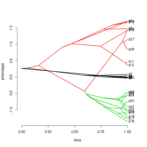
Now that the data are simulated, we can input the appropriate model. First, we need to define a likelihood. I assume that the user will provide the likelihood function. The only requirement is that the likelihood function take in a bayou formatted parameter list and a bayou cache object and return a list with the element '$loglik'.
Let's wrap OUwie's OUMV model into bayou. We're going to use OUwie's likelihood function 'OUwie.fixed'. I'm sure the OUwie developers never intended this to be used in an MCMC, so this is going to be slow and not optimized for bayou.
Note: the cache object is simply a list with a bunch of pre-calculated information about the tree and data. These are useful to calculate once so that subsequent calculations during the MCMC are faster. bayou generates the cache object during the initialization step of the MCMC by calling '.prepare.ou.univariate'.
cache <- bayou:::.prepare.ou.univariate(tt, dd, SE=0)
require(OUwie)
ouwie.lik <- function(pars, cache, X, model="custom"){
  ouwie.pars <- bayou2OUwie(pars, cache$phy, dat=X)
  # Here I use capture.output to suppress OUwie's printing to screen
  capture.output(ouwie.out <<- OUwie.fixed(ouwie.pars$tree, ouwie.pars$dat, model="OUMV", root.station = FALSE, alpha = rep(pars$alpha, pars$ntheta),
                           sigma.sq = exp(pars$sig2), theta=c(pars$theta[1], pars$theta))) #Note that we set the root at the optimum...
  out <- list(loglik=ouwie.out$loglik[1,1])
  return(out)
}
Check and see if it works:
pars <- list(alpha=1, sig2=log(c(1,1,1)), k=2, ntheta=3, theta=c(0,4,4), sb=sample(1:nrow(tt$edge), 2, replace=FALSE), loc=c(0,0), t2=2:3)
ouwie.lik(pars, cache, dd)
## $loglik
## [1] -29.69
ouwie.lik(parsT, cache, dd)## $loglik
## [1] -1.426
Now we need to define a model object for bayou so it knows how to treat the model. It is specified by providing a list of the following items:
- moves - A list of the names of the move functions to use. These may be custom functions as well.
- control.weights - A list giving the relative frequency of each move type
- D - A list giving the tuning weights supplied to each move. NOTE: for the tuning of K, you need to provide a tuning parameter for each of the rjpars!
- parorder - A vector giving the order in which the parameters should be returned (arbitrary preference)
- rjpars - A vector of the parameter names which will be split at each point in the phylogeny
- shiftpars - A vector of the parameters governing the shift locations (this probably should not ever change as of now)
- monitor.fn - A printing function to summarize the pars vector (optional)
- lik.fn - The likelihood function
Defining a monitor function is a little tricky right now, we'll get to it later, for now, we'll just make sure the MCMC doesn't print anything.
model.OUMV <- list(moves = list(alpha=".multiplierProposal", sig2=".vectorSlidingWindow", k=".splitmergebd", theta=".adjustTheta", slide=".slide2"),
                      control.weights = list(alpha=2, sig2=3, theta=3, slide=2, k=10),
                      D = list(alpha=2, sig2=5, k = c(1, 1), theta=2, slide=1),
                      parorder = c("alpha", "sig2", "k", "ntheta", "theta"),
                      rjpars = c("sig2", "theta"),
                      shiftpars = c("sb", "loc", "t2"),
                      lik.fn = ouwie.lik)
Now we define the prior:
prior <- make.prior(tt, plot.prior = TRUE, dists=list(dalpha="dhalfcauchy", dsig2="dnorm", dsb="dsb",
                                                       dk="cdpois", dtheta="dnorm", dloc="dunif"),
                        param=list(dalpha=list(scale=1), dsig2=list(mean=-1, sd=2), dk=list(lambda=10, kmax=20),
                                   dsb=list(bmax=1,prob=1), dtheta=list(mean=0, sd=1), dloc=list(min=0, max=1)),
                            model="custom")
prior(pars, cache) # Test the prior function.## [1] -38.61
We are now ready to run our model. We will need to define our starting parameters since bayou doesn't yet know how to simulate for arbitrary models. We'll just use the values we've been using so far.
testmcmc <- bayou.makeMCMC(tt, dd, model=model.OUMV, prior=prior, startpar=pars, new.dir=TRUE, outname="oumvtest", plot.freq=NULL, ticker.freq=10000, samp = 20)Let's run for 1000 generations just to test it out.
testmcmc$run(1000)
chain <- testmcmc$load()
summary(chain)
## bayou MCMC chain: 1000 generations
## 204 samples, first 1 samples discarded as burnin
##
##
## Summary statistics for parameters:
## Mean SD Naive SE Time-series SE Effective Size
## lnL -24.07667 1.4426 0.10100 0.14327 101.39
## prior -20.96256 4.8479 0.33942 0.35666 184.75
## alpha 0.27725 0.2344 0.01641 0.02520 86.55
## k 1.35294 0.7381 0.05168 0.06025 150.09
## ntheta 2.35294 0.7381 0.05168 0.06025 150.09
## root.sig2 0.07954 0.1699 0.01189 0.02530 45.08
## root.theta 0.26603 0.3708 0.02596 0.01824 413.15
## all sig2 -0.06109 0.5951 NA NA NA
## all theta 0.32522 1.1643 NA NA NA
##
##
## Branches with posterior probabilities higher than 0.1:
## pp magnitude.of.theta2 naive.SE.of.theta2 rel.location
## 20 0.5686 -0.11069 0.14054 0.50911
## 10 0.2549 0.09093 0.09353 0.44625
## 30 0.2157 0.29788 0.12552 0.07225
## 22 0.1078 3.05568 0.19801 0.07045
Now, we've only run for 1000 generations and we don't have a monitor function, so it will break the MCMC when we get to a point where it prints to the screen according to 'ticker.freq'. Let's make a monitor function and redo the analysis. The inputs must ALWAYS be as below (i= generation, lik= likelihood, pr= prior, pars= parameter list, accept= whether accepted, accept.type= proposal type, j= a counter to reprint header names)
model.OUMV$monitor.fn <- function(i, lik, pr, pars, accept, accept.type, j){
  names <- c("gen", "lnL", "prior", "alpha","sig2", "theta","k") #The parameters we want to print
  string <- "%-8i%-8.2f%-8.2f%-8.2f%-8.2f%-8.2f%-8i" #The types of each parameter
  acceptratios <- tapply(accept, accept.type, mean)
  names <- c(names, names(acceptratios))
  if(j==0){
    cat(sprintf("%-7.7s", names), "\n", sep=" ")
  }
  cat(sprintf(string, i, lik, pr, pars$alpha, pars$sig2[1], pars$theta[1], pars$k), sprintf("%-8.2f", acceptratios),"\n", sep="")
}
Let's remake and see if it works.
mymcmc <- bayou.makeMCMC(tt, dd, SE=0, model=model.OUMV, prior=prior, startpar=pars, new.dir=TRUE, outname="oumvtest", plot.freq=NULL, ticker.freq=100, samp = 20)Run it again.
mymcmc$run(10000)## gen lnL prior alpha sig2 theta k .alpha birth.k death.k .sig2 .theta U0.slid
## 100 -24.12 -13.72 0.82 0.14 0.34 0 0.70 0.00 1.00 0.33 0.61 1.00
## 200 -24.21 -13.34 0.32 0.45 0.02 0 0.67 0.00 1.00 0.21 0.56 1.00
## 300 -25.52 -13.56 0.46 0.73 0.17 0 0.62 0.00 1.00 0.19 0.52 1.00
## 400 -23.31 -21.22 0.09 0.04 0.37 1 0.68 0.01 1.00 0.24 0.51 1.00
## 500 -10.85 -19.86 0.16 0.07 -0.38 1 0.68 0.01 0.67 0.27 0.55 1.00
## Error: non-conformable arguments
chain <- mymcmc$load()
summary(chain)
## bayou MCMC chain: 520 generations
## 54 samples, first 1 samples discarded as burnin
##
##
## Summary statistics for parameters:
## Mean SD Naive SE Time-series SE Effective Size
## lnL -22.0518 5.7015 0.77587 2.13481 7.133
## prior -18.3615 6.2484 0.85030 1.75345 12.698
## alpha 0.5104 0.3643 0.04958 0.09702 14.101
## k 0.6667 0.7770 0.10574 0.27381 8.053
## ntheta 1.6667 0.7770 0.10574 0.27381 8.053
## root.sig2 0.2379 0.2829 0.03850 0.04588 38.021
## root.theta 0.1820 0.2881 0.03921 0.03921 54.000
## all sig2 -1.0888 2.3781 NA NA NA
## all theta 0.3433 1.0844 NA NA NA
##
##
## Branches with posterior probabilities higher than 0.1:
## pp magnitude.of.theta2 naive.SE.of.theta2 rel.location
## 7 0.2963 -0.26807 0.1492 0.1941
## 55 0.2222 0.07086 0.1633 0.5264
plotSimmap.mcmc(tr$tree, chain, burnin=0)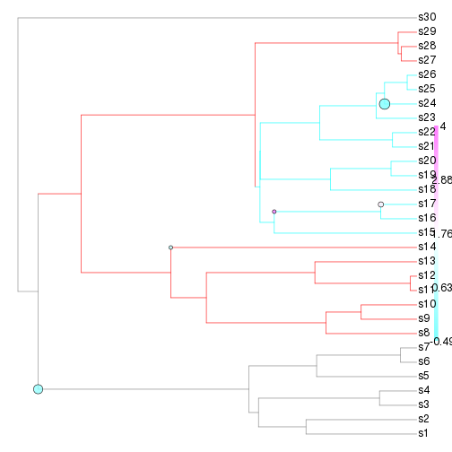
Doesn't look very good so far...whether or not it ever gets the right answer and converges is beyond the scope here, One problem is that OUwie.fixed is pretty slow, so speeding up this function is probably necessary to really give this a good test. Let's try it fixing the location of the shifts to at least make sure we get the right variance estimates:
model.OUMVFixed <- list(moves = list(alpha=".multiplierProposal", sig2=".vectorSlidingWindow", theta=".adjustTheta"),
                   control.weights = list(alpha=1, sig2=1, theta=1, k=0),
                   D = list(alpha=2, sig2=5, theta=2),
                   parorder = c("alpha", "sig2", "k", "ntheta", "theta"),
                   rjpars = c("sig2", "theta"),
                   shiftpars = c("sb", "loc", "t2"),
                   monitor.fn = model.OUMV$monitor.fn,
                   lik.fn = ouwie.lik)
startpar.fixed <- parsT
fixed.hypothesis <- parsT[c("sb", "t2", "loc")]
startpar.fixed$alpha <- 1; startpar.fixed$sig2 <- c(1,1,1); startpar.fixed$theta=c(2,2,2)

prior.fixed <- make.prior(tt, plot.prior = TRUE, dists=list(dalpha="dhalfcauchy", dsig2="dnorm", dsb="fixed",
                                                            dk="fixed", dtheta="dnorm", dloc="dunif"),
                          param=list(dalpha=list(scale=1), dsig2=list(mean=-1, sd=2), dtheta=list(mean=0, sd=1), dloc=list(min=0, max=1)),
                          fixed=fixed.hypothesis)
mymcmc.fixed <- bayou.makeMCMC(tt, dd, SE=0, model=model.OUMVFixed, prior=prior.fixed, startpar=startpar.fixed,
                               new.dir=TRUE,  outname="oumvfixed", plot.freq=NULL, ticker.freq=100, samp = 20)


mymcmc.fixed$run(10000)
## gen lnL prior alpha sig2 theta k .alpha .sig2 .theta
## 100 -19.34 -11.45 0.93 -1.98 0.26 2 0.63 0.51 0.67
## 200 -4.69 -10.91 0.65 -4.02 0.08 2 0.59 0.40 0.69
## 300 2.14 -15.80 1.92 -3.55 0.05 2 0.56 0.33 0.62
## 400 6.61 -13.70 3.50 -3.69 -0.00 2 0.50 0.30 0.58
## 500 6.98 -15.95 3.12 -4.63 -0.00 2 0.45 0.28 0.51
## 600 5.61 -14.35 5.51 -3.34 0.02 2 0.45 0.31 0.49
## 700 4.24 -15.06 6.16 -2.96 0.02 2 0.42 0.33 0.46
## 800 4.20 -13.88 1.85 -3.90 0.02 2 0.41 0.31 0.43
## 900 4.57 -13.82 1.85 -4.65 0.02 2 0.41 0.30 0.40
## 1000 4.94 -13.58 4.14 -3.65 0.02 2 0.41 0.30 0.38
## 1100 6.82 -15.60 7.90 -4.41 0.02 2 0.40 0.28 0.37
## 1200 4.62 -15.93 6.90 -3.25 0.02 2 0.40 0.29 0.35
## 1300 4.83 -15.99 1.86 -5.23 0.02 2 0.41 0.29 0.35
## 1400 5.61 -14.73 2.33 -4.06 0.02 2 0.39 0.29 0.33
## 1500 4.68 -15.44 2.86 -5.47 0.02 2 0.38 0.28 0.32
## 1600 4.86 -14.28 5.08 -3.60 0.02 2 0.38 0.28 0.31
## 1700 2.29 -13.77 3.17 -4.73 0.02 2 0.38 0.29 0.30
## 1800 4.16 -14.63 2.82 -3.96 0.01 2 0.37 0.29 0.31
## 1900 5.45 -14.75 2.91 -3.70 0.01 2 0.37 0.30 0.31
## 2000 7.30 -15.90 2.97 -5.09 0.01 2 0.38 0.29 0.31
## 2100 2.39 -14.60 4.60 -3.14 0.01 2 0.38 0.30 0.32
## 2200 3.37 -14.33 7.44 -3.29 0.01 2 0.38 0.30 0.31
## 2300 5.59 -14.47 2.24 -5.23 0.01 2 0.38 0.30 0.31
## 2400 8.06 -15.01 4.84 -4.49 0.01 2 0.38 0.29 0.30
## 2500 6.96 -14.80 8.70 -2.83 0.01 2 0.37 0.29 0.29
## 2600 -2.46 -11.88 0.68 -5.10 0.01 2 0.38 0.29 0.29
## 2700 1.36 -13.87 1.39 -5.06 0.00 2 0.39 0.29 0.30
## 2800 7.29 -15.26 7.06 -3.67 0.00 2 0.39 0.29 0.29
## 2900 5.71 -14.29 2.08 -4.54 0.00 2 0.39 0.29 0.29
## 3000 5.75 -13.62 2.99 -3.92 0.01 2 0.39 0.29 0.29
## 3100 8.13 -14.72 5.55 -4.03 0.01 2 0.39 0.29 0.28
## 3200 5.87 -13.72 3.51 -4.09 0.01 2 0.38 0.29 0.29
## 3300 2.66 -15.52 5.07 -5.24 0.01 2 0.38 0.30 0.29
## 3400 5.37 -15.33 6.69 -3.06 0.01 2 0.38 0.30 0.29
## 3500 4.76 -14.40 4.95 -3.62 0.01 2 0.38 0.30 0.28
## 3600 6.48 -13.85 2.96 -3.83 0.01 2 0.38 0.30 0.28
## 3700 0.13 -14.90 1.33 -4.57 -0.04 2 0.38 0.30 0.28
## 3800 5.24 -13.94 2.87 -3.52 -0.01 2 0.38 0.30 0.29
## 3900 -0.09 -14.19 1.83 -3.67 -0.10 2 0.38 0.30 0.29
## 4000 -3.25 -13.34 1.45 -2.54 -0.10 2 0.38 0.30 0.29
## 4100 -6.40 -13.15 1.31 -2.54 -0.10 2 0.38 0.29 0.29
## 4200 6.66 -14.57 3.46 -4.53 0.02 2 0.38 0.29 0.29
## 4300 5.69 -13.74 3.97 -3.13 0.02 2 0.38 0.30 0.29
## 4400 4.40 -13.89 4.96 -4.03 0.02 2 0.38 0.30 0.29
## 4500 6.77 -14.88 6.26 -3.41 0.02 2 0.37 0.30 0.29
## 4600 5.68 -14.40 5.79 -3.61 0.02 2 0.37 0.30 0.28
## 4700 3.12 -13.91 3.97 -4.29 0.02 2 0.37 0.30 0.28
## 4800 7.05 -14.62 3.56 -3.79 0.02 2 0.37 0.30 0.28
## 4900 2.87 -13.54 4.44 -3.06 0.01 2 0.37 0.30 0.28
## 5000 6.32 -14.62 5.08 -3.67 0.01 2 0.37 0.30 0.28
## 5100 8.32 -15.05 6.51 -3.82 0.02 2 0.36 0.30 0.27
## 5200 7.42 -15.21 7.59 -3.44 0.02 2 0.36 0.30 0.27
## 5300 5.09 -14.55 2.96 -3.81 0.05 2 0.36 0.30 0.27
## 5400 5.50 -14.65 2.42 -4.30 0.05 2 0.36 0.30 0.28
## 5500 2.90 -14.39 2.59 -3.16 -0.03 2 0.36 0.30 0.28
## 5600 -2.96 -16.01 1.19 -2.91 0.09 2 0.36 0.30 0.28
## 5700 3.40 -15.33 1.89 -4.36 0.01 2 0.36 0.29 0.28
## 5800 6.29 -16.66 1.87 -4.56 0.01 2 0.37 0.30 0.28
## 5900 4.00 -14.86 3.27 -5.22 -0.02 2 0.36 0.30 0.28
## 6000 5.65 -14.36 3.26 -4.23 -0.02 2 0.37 0.30 0.28
## 6100 6.75 -14.92 6.14 -3.57 0.03 2 0.37 0.30 0.28
## 6200 5.08 -14.85 5.06 -3.50 0.03 2 0.37 0.30 0.28
## 6300 4.98 -14.62 4.57 -4.34 0.03 2 0.37 0.30 0.28
## 6400 2.67 -16.15 1.73 -3.54 0.03 2 0.37 0.30 0.28
## 6500 6.27 -15.24 2.62 -4.46 0.03 2 0.37 0.30 0.28
## 6600 5.48 -17.11 1.90 -5.19 0.03 2 0.37 0.30 0.29
## 6700 7.25 -15.61 2.65 -4.89 0.02 2 0.37 0.30 0.29
## 6800 6.79 -13.87 3.52 -4.23 0.02 2 0.37 0.30 0.28
## 6900 8.25 -14.68 4.41 -4.12 0.02 2 0.37 0.30 0.28
## 7000 6.22 -14.89 5.02 -4.34 0.02 2 0.36 0.29 0.28
## 7100 3.58 -13.51 5.06 -2.72 0.02 2 0.36 0.29 0.28
## 7200 5.21 -14.77 6.37 -3.89 0.02 2 0.36 0.30 0.28
## 7300 3.56 -14.81 7.96 -3.09 0.02 2 0.36 0.30 0.28
## 7400 2.95 -13.53 2.73 -3.91 0.02 2 0.36 0.30 0.28
## 7500 3.93 -14.63 3.10 -4.87 0.01 2 0.36 0.30 0.28
## 7600 3.70 -14.33 4.44 -3.46 0.01 2 0.36 0.30 0.28
## 7700 6.01 -15.28 3.72 -4.48 0.01 2 0.36 0.30 0.28
## 7800 6.21 -13.94 4.50 -4.05 0.02 2 0.36 0.30 0.28
## 7900 6.71 -14.44 5.02 -4.42 0.02 2 0.36 0.30 0.28
## 8000 7.11 -14.77 3.57 -4.64 0.02 2 0.36 0.30 0.28
## 8100 7.19 -15.21 4.76 -4.50 -0.01 2 0.36 0.30 0.28
## 8200 6.85 -15.10 4.76 -4.22 -0.01 2 0.36 0.30 0.28
## 8300 7.45 -14.85 3.53 -4.22 -0.01 2 0.36 0.29 0.28
## 8400 4.20 -13.71 2.38 -4.22 -0.01 2 0.36 0.29 0.28
## 8500 7.28 -14.59 5.26 -4.18 -0.01 2 0.36 0.29 0.28
## 8600 3.60 -13.86 2.53 -4.02 -0.01 2 0.36 0.29 0.28
## 8700 7.11 -15.08 2.85 -4.22 0.02 2 0.36 0.29 0.28
## 8800 1.04 -14.55 3.84 -2.57 0.02 2 0.35 0.29 0.28
## 8900 5.55 -13.92 3.67 -4.47 0.02 2 0.35 0.29 0.28
## 9000 7.65 -14.61 4.16 -4.70 0.02 2 0.35 0.29 0.27
## 9100 7.43 -14.66 4.46 -4.02 0.02 2 0.35 0.29 0.27
## 9200 4.97 -14.87 2.33 -5.10 0.02 2 0.36 0.29 0.28
## 9300 5.75 -14.20 4.54 -4.01 0.02 2 0.36 0.29 0.28
## 9400 4.72 -13.89 3.25 -3.53 -0.01 2 0.36 0.29 0.28
## 9500 5.29 -15.62 1.65 -4.53 -0.01 2 0.36 0.29 0.28
## 9600 3.53 -16.26 6.59 -4.32 -0.01 2 0.36 0.29 0.28
## 9700 4.94 -14.52 3.46 -3.29 -0.01 2 0.36 0.29 0.28
## 9800 4.79 -15.76 5.13 -4.55 -0.01 2 0.35 0.29 0.28
## 9900 5.08 -14.78 2.13 -4.71 -0.01 2 0.35 0.29 0.28
## 10000 1.73 -13.45 3.76 -3.24 -0.01 2 0.35 0.29 0.28
chain <- mymcmc.fixed$load()

# Plot to see if sigma^2 is estimated ok:
sig2post <- do.call(rbind, chain$sig2)
plot(c(0, nrow(sig2post)),c(min(sig2post)-1, max(sig2post)+1), type="n", xlab="mcmc sample", ylab="log sigma^2")
lapply(1:ncol(sig2post), function(x) lines(1:nrow(sig2post), sig2post[,x], col=x+1))abline(h=parsT$sig2, col=1+(1:ncol(sig2post)))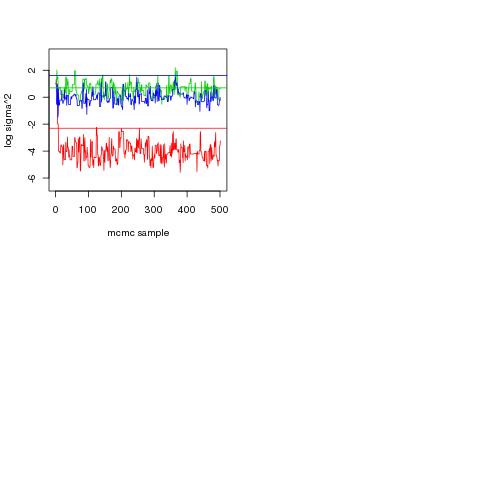
This seems pretty reasonable, given that the trees are pretty small.
That's all, any feedback is greatly appreciated!!