InterfaceFeatures
The DASH Windows interface enables you to carry out all the necessary steps for structure solution. This section explains the layout of the main window and the various input and output files.
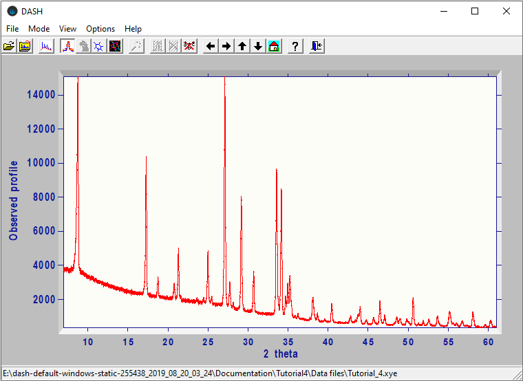
This is an example of the main window after reading in an X-ray diffraction pattern of laboratory data for Decafluoroquaterphenyl (Smrcok, L. et al., Z. Kristallogr. (2001) 216, 63-66):
There are three ways of accessing most functions in DASH:
-
Through the Wizard, use of the Wizard is highly recommended.
-
From the top level menu: File, Mode, View, Options and Help.
-
Using the Icon buttons, which provide access to functions with one mouse click.
The main window displays the experimental diffraction profile and, when applicable, the background, any selected peaks, the calculated profile, the difference profile and the cumulative χ2, with various colour coding conventions. The path to the current diffraction data file is shown at the bottom left of the status bar. The coordinates of the current mouse-cursor position and the h, k, l values of the peak nearest to the mouse cursor are shown at the bottom right of the status bar.
To input a powder diffraction file, it is recommended that you use the option View data / determine peak positions from the main Wizard window (see The DASH Wizard). Alternatively, you can use the Wizard option Preparation for Pawley refinement, or click on the following icon:

This leads to a pop-up window that shows all files in the selected directory with an extension that match those of the file types that can be read by DASH. These include:
-
.raw - Bruker (more information about this file type is given below)
-
.raw - STOE (more information about this file type is given below)
-
.rd and .sd - Philips
-
.udf
-
.uxd
-
.xye
-
.cpi - Sietronics
-
.mdi - Materials Data Inc.
-
.pod - Daresbury
-
.x01 - Bede
-
.txt - ThermoARL
-
.asc - Rigaku
Simply:
-
Click on the file icon/filename (this places the filename in the box).
-
Click on Open.
When a Bruker .raw file is opened, DASH scans the file for data ranges. When only one is found, it is loaded, but when more than one is found, the data ranges to be summed can be selected through the following dialogue window:

By default all data ranges are selected and clicking OK reads in all data ranges.
DASH sums the data ranges as follows:
-
Per 2θ value (= data point), the number of raw counts and the number of seconds that has been counted for is stored.
-
The combined list of 2θ values from all data ranges is sorted in ascending order.
-
If two 2θ values are closer together than the smallest 2θ step used in any of the patterns being summed they are merged by summing their raw numbers of counts, summing their counting times and averaging their 2θ values. This process is repeated until the original smallest step size is restored.
-
The intensities are scaled to Counts Per Second by dividing the total raw number of counts per 2θ value by the total number of seconds counted for that 2θ value. The ESDs are calculated as (total raw number of counts)1/2 / (total number of seconds counted for).
It is possible to implement an optimised data collection strategy (see Optimising Use of Data Collection Time) using multiple data ranges in Bruker .raw files. In an optimised data collection strategy data points at higher 2θ, which on average have less intensity, are measured longer than data points at lower 2θ. The Variable Counting Time scheme used for the above file would have been:
| 2θ range | Counting time (seconds per step) |
|---|---|
| 5.0 - 15.0 | 0.5 |
| 15.0 - 25.0 | 1.0 |
| 25.0 - 35.0 | 2.0 |
| 35.0 - 45.0 | 4.0 |
| 45.0 - 55.0 | 8.0 |
| 55.0 - 65.0 | 16.0 |
The third step is performed to smooth the seams between two adjacent data ranges, but it also allows reading in of data that has been collected using the following Variable Counting Time scheme, entirely equivalent to the previous one:
| 2θ range | Counting time (seconds per step) |
|---|---|
| 5.0 - 65.0 | 0.5 |
| 15.0 - 65.0 | 0.5 |
| 25.0 - 65.0 | 1.0 |
| 35.0 - 65.0 | 2.0 |
| 45.0 - 65.0 | 4.0 |
| 55.0 - 65.0 | 8.0 |
DASH recognises two formats of diffraction data within the file type with extension .xye (the file should be a normal ASCII text file):
-
2θ, counter reading, estimated standard deviation of the count.
-
2θ, counter reading.
If no standard deviation is given in the input file DASH recognises this and sets the standard deviation to be the square root of the count. The start of an example file, where the diffractometer step size is 0.004o 2θ, is given below:
5.000 81.96 10.952
5.004 71.25 10.284
5.008 72.40 10.343
5.012 76.87 10.661
5.016 63.58 9.695
Optionally, the wavelength can be included in the file as the very first line.
The main window shows the diffraction data plotted as observed counts versus 2θ. There are numerous keyboard and mouse facilities for selecting ranges of 2θ, scaling of peak height, and generally zooming into a region of the profile for closer examination (see Preliminary Inspection of Profile). The next stage for consideration is removal of the background from the data (see Removing the Background from Diffraction Data).
It is recommended that the background is subtracted through the Wizard (see The DASH Wizard). Alternatively the background can be subtracted choosing the following icon from the menu bar:

The method of background removal is a Monte Carlo low-pass filter, which has advantages of being mathematically robust. It is recommended that you let DASH take care of the background subtraction at this stage. If you choose to leave the background fitting to later, it will be included in the Pawley fitting process, using a shifted Chebyshev polynomial (see Choosing Peaks Prior to Initial Pawley Fitting: an Example).
Note: If your data set is of laboratory origin, or there is noticeable non-uniform background then it is best to remove the background using the Monte Carlo method. Poor quality data sets that are not background-subtracted at this stage (i.e. sets where the discrimination between peaks and background is poor) can give rise to problems at the Pawley Fitting stage, due to correlation between the polynomial background and the very weak intensities.

-
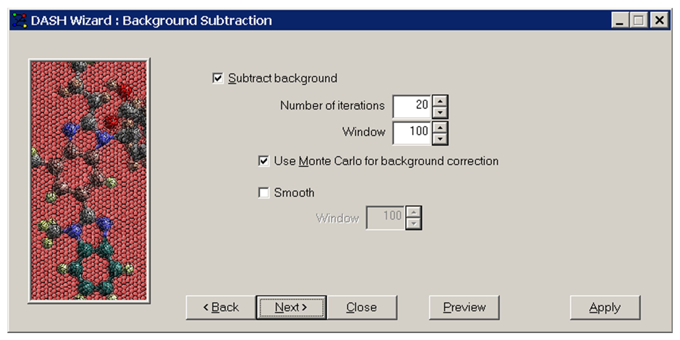
The pass filter value is set at 100 by default.
-
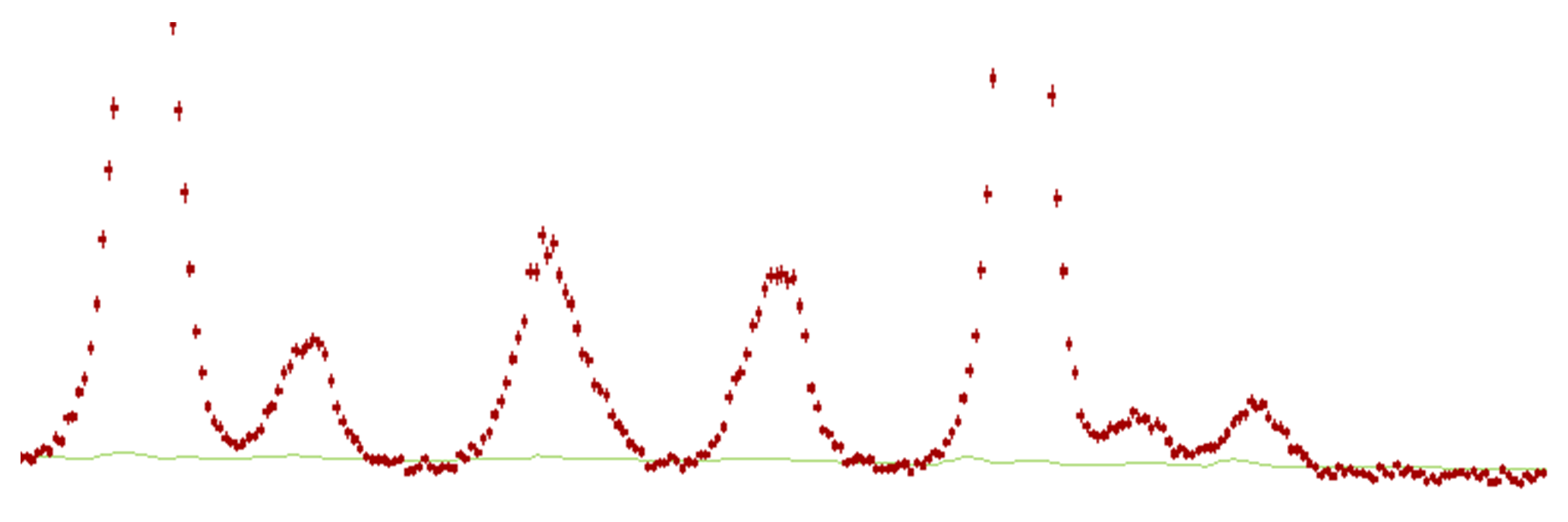
Select Preview to run the fitting; the display now shows the background fitted as a green line. Check that it looks reasonable and is not removing any significant intensity from the peaks. A close-up view of a fitted background on a laboratory data set is given below:
-
If you are not happy with the background you can try smaller or larger values of the Low-pass filter window size. This value is related to the number of data points per degree, and larger values tend to give a smoother, more featureless background, whilst smaller values allow the program to give a varying background more accurately. A closer look at the above example shows that whilst the background estimate is excellent there are a few ripples in the background line. Increasing the low-pass filter window size and applying it will smooth out these ripples. Select a value that suits your data, remembering to look closely at the high angle estimates, where the peaks are weak.
-
Select Accept if satisfactory; DASH now subtracts the background from the data, as will be seen in the updated display.
DASH keeps a record of progress while one is working on a chosen set of diffraction data. When you start a new project, the only item in the directory will be your diffraction data file. After indexing the cell, and extracting intensities by the Pawley fit procedure, DASH creates a file with extension .sdi that is then known as the Pawley-Fit file (see Pawley-Fit File: an Example). This contains all the information needed for the last stage of the DASH process, i.e. structure solution using a molecular model.
The default name is based on the diffraction data file; e.g. for a compound called hydrochlorothiazide, we might have a data file hct.xye, producing a Pawley-Fit file hct.sdi. If you had a second set of experimental data for hydrochlorothiazide, e.g. hctnew.xye and chose this as the input file, DASH would create a new Pawley-Fit file called, by default, hctnew.sdi, but you can choose the names as you wish.
The Pawley-Fit file contains the full file names for various types of data that are created by DASH as the result of the Pawley refinement. It is not essential to know the details of these files, but it is important to be aware of the data files that are used by the structure solution process. Each line lists a file or some data that is identified by a keyword:
-
TIC: Tick-mark file, with hkl and 2θ positions of extracted intensities.
-
HCV: Extracted hkl intensities and reflection correlations.
-
PIK: Background-subtracted profile.
-
RAW: File name for the original data file.
-
DSL: Data type, wavelength, and peak shape parameters.
-
Cell: the unit cell parameters.
-
SpaceGroup: Space group selected for the Pawley refinement.
-
PawleyChiSq: χ2 fit achieved by the Pawley refinement.
An example of the file hct20.sdi is given below:
TIC .\hct20.tic
HCV .\hct20.hcv
HCV .\hct20.hkl
PIK .\hct20.pik
RAW .\hct20.raw
DSL .\hct20.dsl
Cell 9.93861 8.49849 7.31737 90.0000 111.1896 90.0000
SpaceGroup 38 4:b P 1 21 1
PawleyChiSq 2.41
After you have proceeded with the cell indexing step and choice of space group, there are options for viewing the current peak list etc. These items are selected from the top-level menu button View, as follows:
-
Diffraction Setup: Type of data, wavelength etc. (see Viewing Diffraction Setup).
-
Peak Positions: 2θ for fitted peaks (see Viewing Peak Positions).
-
Cell Parameters: Cell dimensions, space group etc. (see Viewing Unit Cell Parameters).
-
Peak Widths: Parameters describing peak shape (see Viewing Peak Widths).
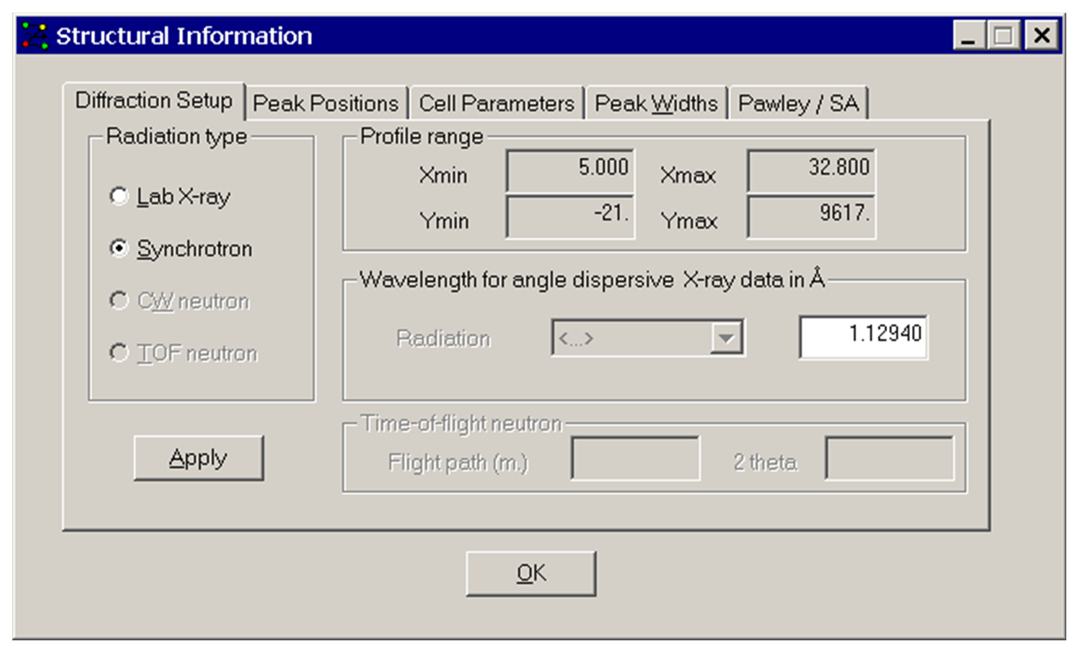
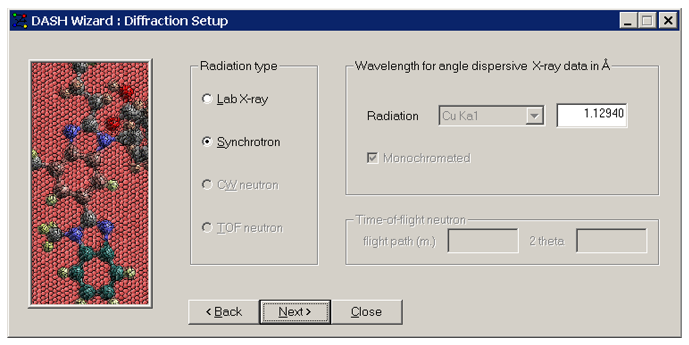
The above Structural Information window appears after selecting Diffraction Setup from the View menu. Information can be entered on:
-
Radiation type: Laboratory or Synchrotron (DASH does not currently handle neutron data).
-
Profile Range: This is for information only.
-
Wavelength: The radiation wavelength used is entered here. For a synchrotron data set, you must enter the wavelength in the entry field. For laboratory data, you can either type the wavelength or use the pull down menu to select the appropriate radiation type.
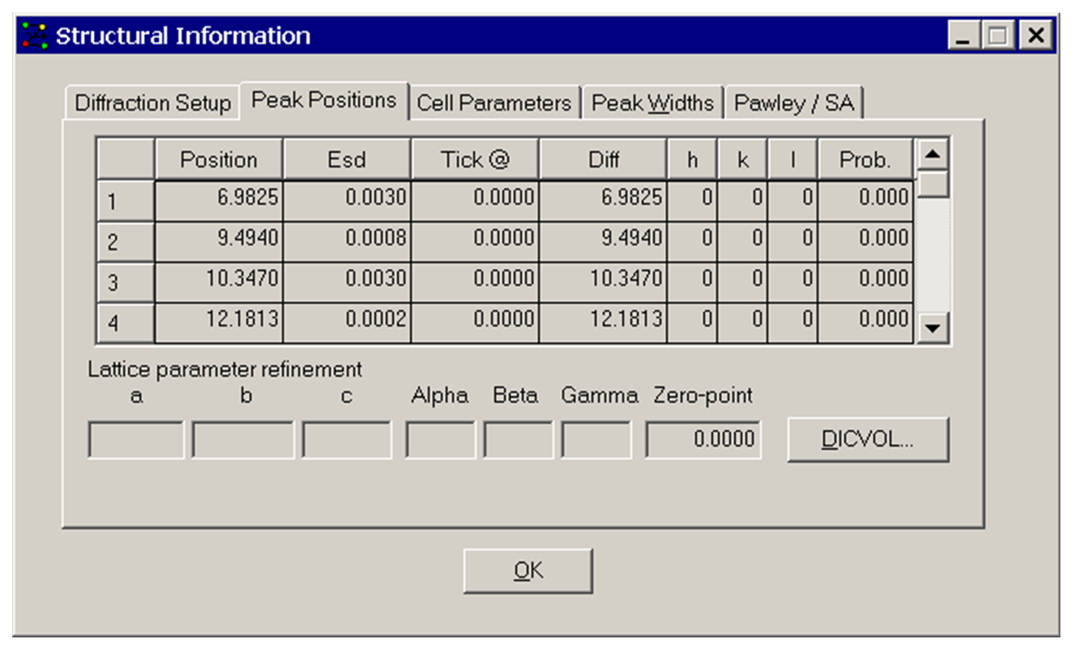
The above Structural Information window appears after selecting Peak Positions from the View menu. This example shows a list of peaks fitted ready for cell indexing.
-
Position: the peak position in 2θ.
-
ESD: the estimated standard deviation of the position in 2θ.
-
Tick: the 2θ position calculated from unit cell (once entered).
-
Diff: the difference between the observed position and the tick-mark.
-
hkl: after unit cell indexing these are the Miller indices assigned to the peak.
-
Prob: probability of correctness of assignment.
-
Lattice parameters and Zero-point: These fields are filled in after a Pawley refinement, or when an on-the-fly cell refinement has been performed. These are display fields only.
-
The DICVOL... button can be used to create an input file ready for the DICVOL indexing program, after fitting a number of peaks (see Indexing).

The above Structural Information window appears after selecting Cell Parameters from the View menu. This example shows a cell and space group ready for input to the Pawley Refinement:
-
a, b, c: unit cell lengths in units of Angstroms.
-
Alpha, beta, gamma: unit cell angles (degrees).
-
Volume: calculated volume of the unit cell (cubic Angstroms)
-
Zero-point: zero-point error of the powder pattern in degrees 2 theta (if known).
-
Crystal System: a list of the crystal systems.
-
Space Group: a list of space group symbols in various settings.
-
Clicking on the following icon clears the unit cell parameters:


The above Structural Information window appears after selecting Peak Widths from the View menu. There are six tabs that allow you to access details of the peak description parameters. These fields are for display only. The fields are populated once a few peaks have been fitted, as reliable peak shape parameters have been calculated by this stage. Inspection of the values can be useful in deciding which peak shape parameters (if any) need to be varied in a Pawley refinement (see Reflection-Intensity Fitting).
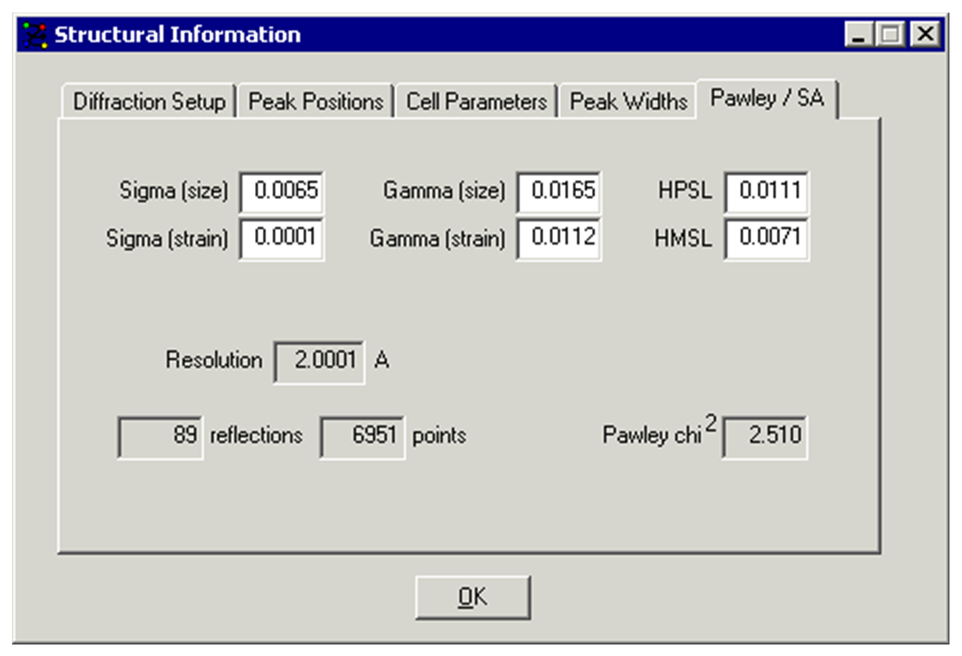
The above Structural Information window appears after selecting Pawley / SA from the View menu. This example shows several pieces of information about the last Pawley refinement. It is possible to manually enter values that will be used for subsequent Pawley refinements, but this should not usually be necessary.
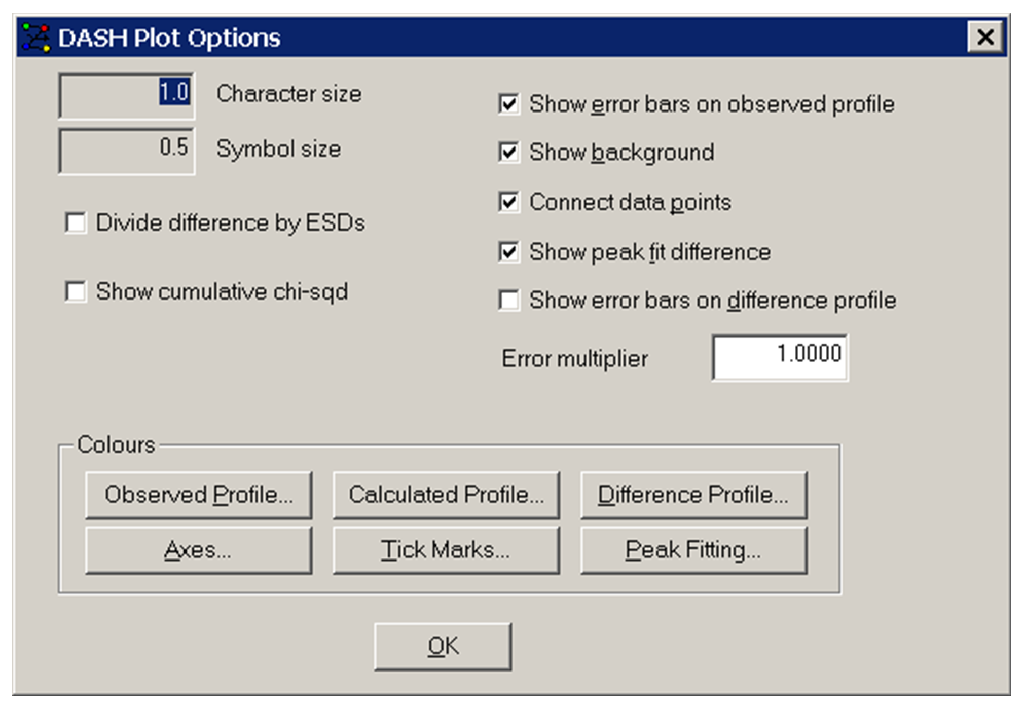
The DASH Plot Options window appears after selecting Options from the top-level menu:
-
Character size: not currently active.
-
Symbol size: not currently active.
-
Show Error bars on Observed Profile: display of the error bars on data point may be toggled on and off using this control.
-
Show Background: display of the calculated background may be toggled on and off using this control.
-
Connect data points: display of lines connecting the data points of the powder pattern may be toggled on and off using this control.
-
Show peak fit difference: display of the difference between measured and fitted peaks may be toggled on and off using this control.
-
Show Error Bars on Difference Profile: display of the error bars on a data point in the difference profile may be toggled on and off using this control.
-
Error Multiplier: Used to control the value of the multiplier applied to error bars.
-
Divide difference by ESDs: when ticked, the points of the difference curve are divided by the ESDs of the observed number of counts and multiplied by the average ESD.
-
Show cumulative chi-sqd: display of the cumulative chi-sqd during Pawley refinement and simulated annealing may be toggled on and off using this control.
-
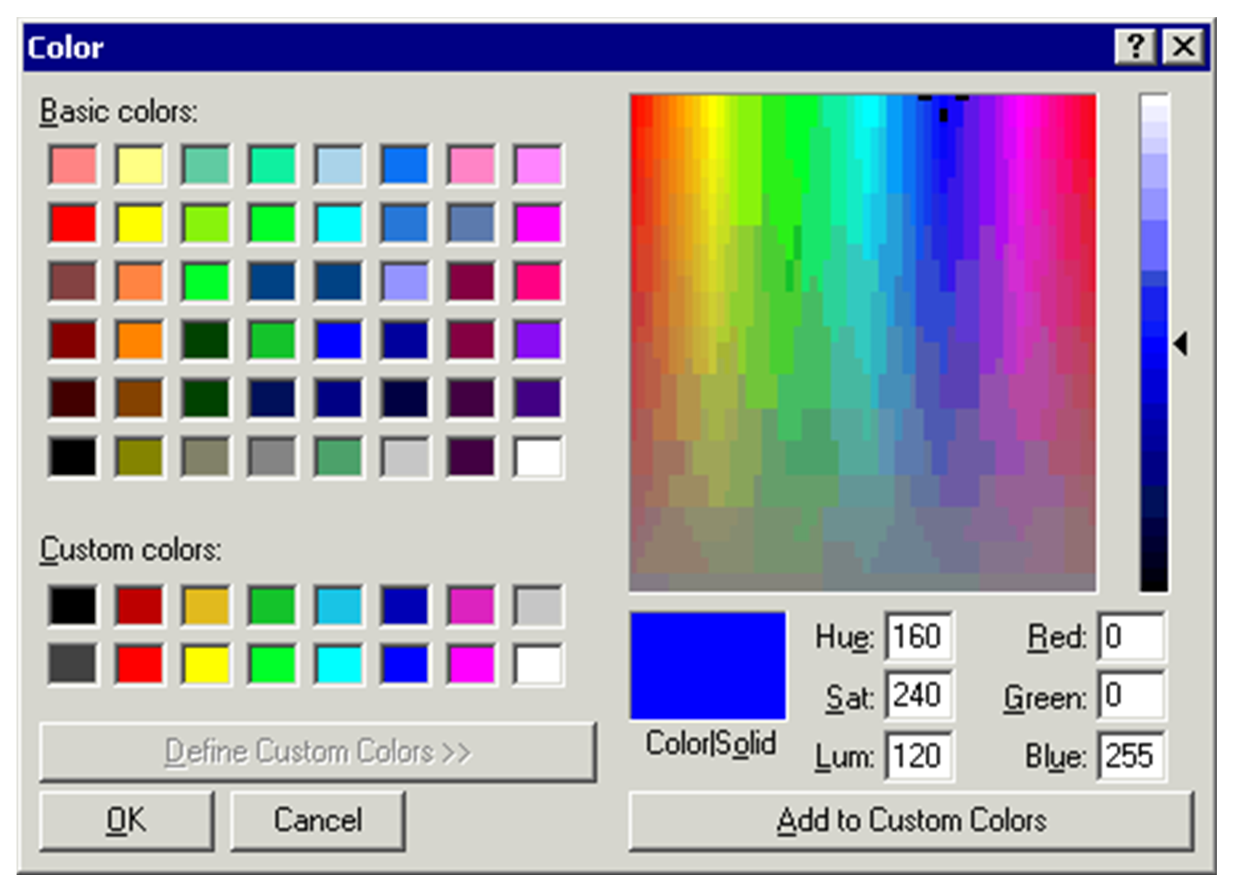
Colours: these buttons may be used to alter the default colours used by DASH for display of the profile. Selecting any one of the buttons brings up a colour chooser, from which you may select a colour by clicking on the appropriate square:
-
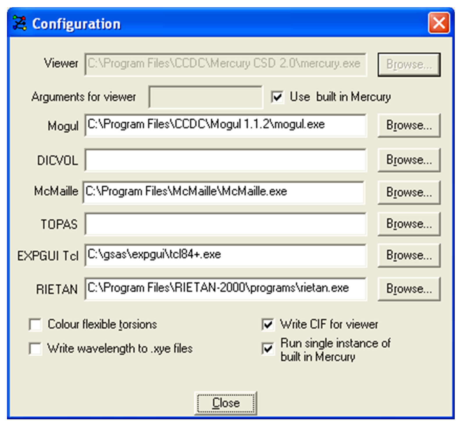
Viewer: the viewer used for viewing Z-matrices and solutions. The viewer will display crystal structures from .cif, .pdb or .mol2 files.
-
Arguments for viewer: If using built-in Mercury the command line argument to load-all-files is supplied by default. This ensures that when .cif files are written for structures to be overlaid, all structures are loaded and displayed simultaneously. If Mercury is used to view structures, supplying the command line argument -client will load each structure selected into a single instance of Mercury. If, within Mercury, the Multiple Structures check box is ticked, the structures will be displayed simultaneously.
-
Mogul: If access to Mogul is available then enter the path to the Mogul executable here or click on the Browse button.
-
DICVOL: If DICVOL04 is available for indexing then enter the path to the DICVOL executable here or click on the Browse button.
-
McMaille: If McMaille is available for indexing then enter the path to the McMaille executable here or click on the Browse button.
-
TOPAS: If TOPAS is available for Rietveld refinement then enter the path to the TOPAS executable or click on the Browse button.
-
EXPGUI Tcl: If GSAS is available for Rietveld refinement then enter the path to the tcl84+.exe (in the expgui folder) here or click on the Browse button.
-
RIETAN: If RIETAN is available for Rietveld refinement then enter the path to the RIETAN executable here or click on the Browse button.
-
Colour flexible torsions: when selected, flexible torsion angles are colour coded when viewing a Z-matrix.
-
Write wavelength to .xye files: If checked the wavelength entered or selected when reading in a powder pattern will be automatically written to the .xye file.
-
Write CIF for Viewer: If checked, individual .cif files will be written for all structures chosen to be overlaid. If using built-in Mercury, these files will be automatically displayed simultaneously. If Mercury is used, the .cif files will be loaded but to display the structures simultaneously, the Multiple Structures dialog has to be invoked.
-
Run single instance of built-in Mercury: When ticked, only one copy of built-in Mercury will be opened and all structures will be loaded into that instance of Mercury. Unticking the check box will cause a fresh copy of built-in Mercury to be opened each time a structure is selected for viewing.
The online version of this user guide is available by clicking the
Help button, the
 icon or by using the keyboard command Ctrl-H. The following features
are available:
icon or by using the keyboard command Ctrl-H. The following features
are available:
-
DASH Help: allows you to view a copy of the current user guide and also provides access to the Tutorials.
-
DASH Tutorials: allows you to view a set of Tutorials for DASH. Clicking on any of the tutorials will cause a window to pop up prompting the user to supply a directory in which to save the files for the specific tutorial. Clicking on the “..” feature will cause the browser to go up a level within the directory structure for navigation purposes.

- About DASH: gives the DASH version number.

The DASH Wizard has been designed to guide you through the structure solution process, which is performed in a series of steps:
-
View data/determine peak positions (see View Data / Determine Peak Positions).
-
Preparation of single crystal data (see Preparation of Single Crystal Data).
-
Simulated annealing structure solution (see Structure Solution).
-
Analyse solutions (see Files saved from multiple runs of SA).
-
Rietveld refinement (see Rietveld Refinement in DASH).
It may be called up at any time by clicking the
 icon in the main window.
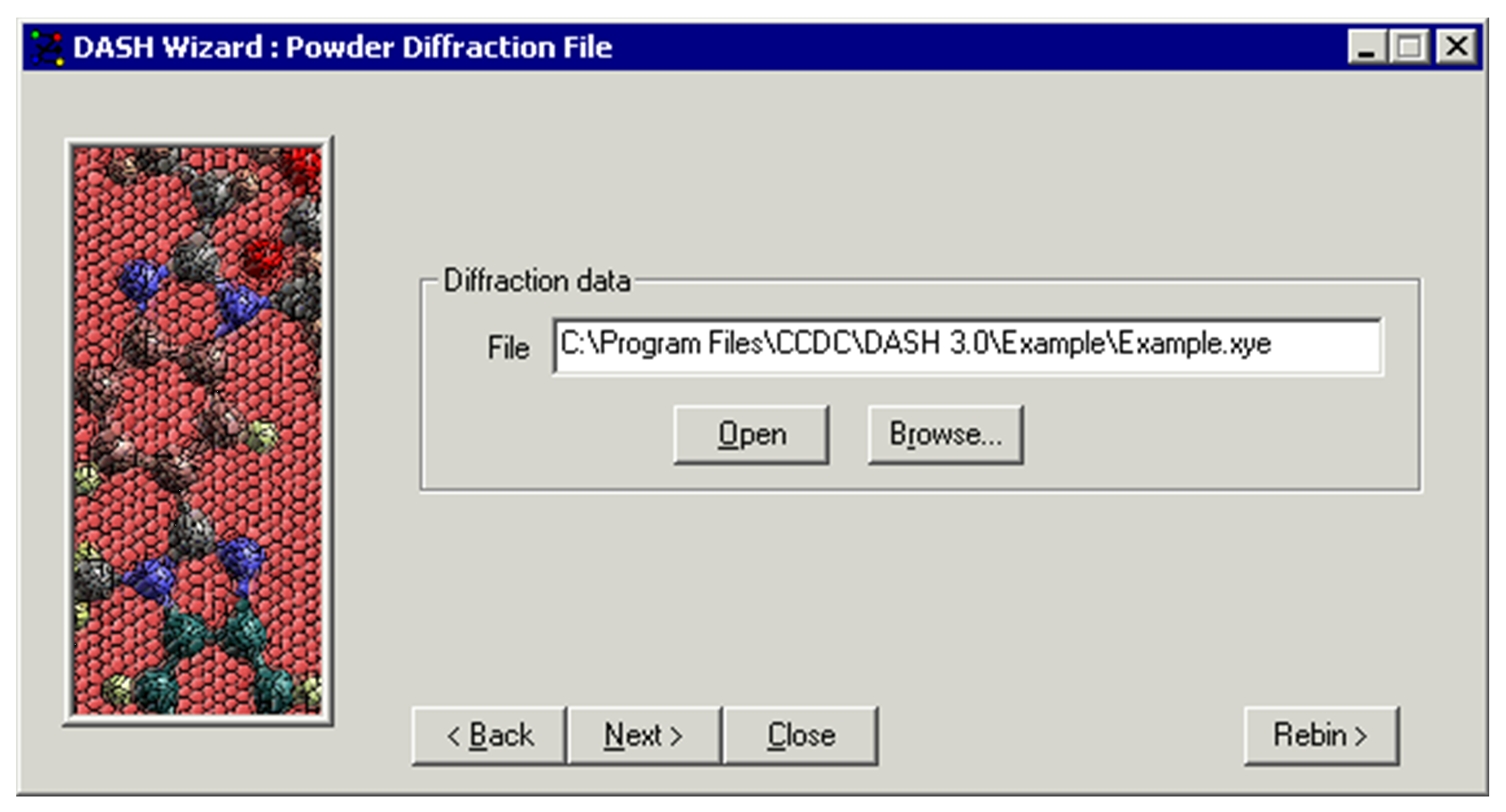
- Select the first option View data / determine peak positions and click Next >.
-
Click Browse...
-
Select a data file, e.g. Example.xye, and the diffraction data will be loaded into DASH and displayed.
-
You are given the opportunity to rebin the data by choosing Rebin >, otherwise click Next >.
-
Check that the radiation type and wavelength have been set correctly.
-
Click Next >.
-
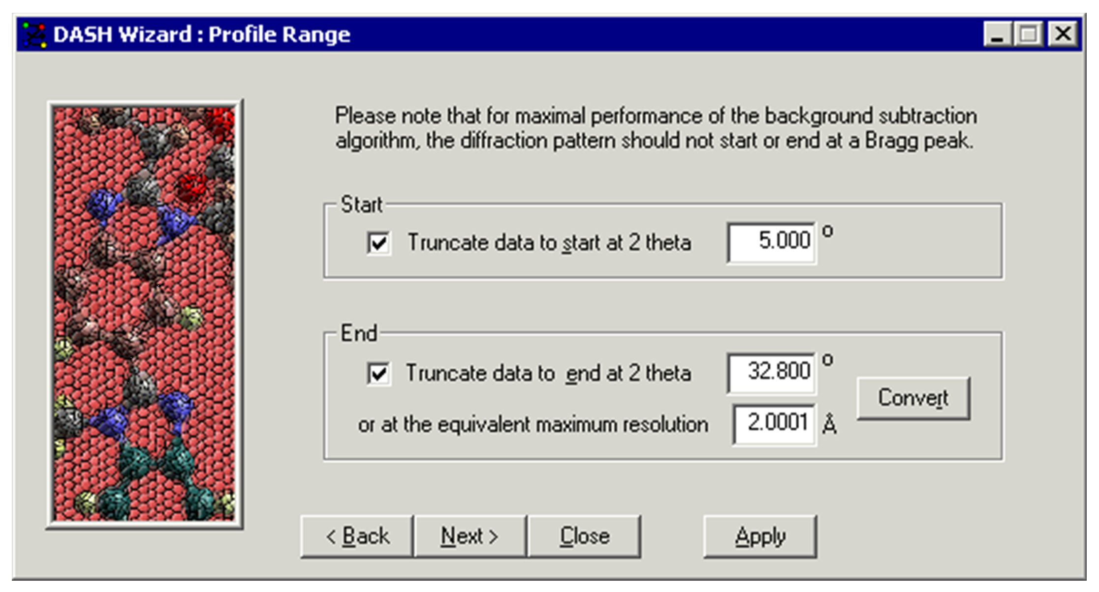
Enter the 2θ angle at which the pattern should be truncated at the beginning. This gives the possibility to remove the part of the pattern affected by the beam stop.
-
Enter the 2θ angle at which the pattern should be truncated at the end. This gives the possibility to truncate the data to a certain resolution (see Truncating the Data).
-
Click Next >.
-
Adjust the width of the window to match the curvature of the background.
-
Smooth: Checking this box will smooth the profile before the background is subtracted, using a window size of x data points, where x is specified in Window. The intensity at point I will be recalculated to be the average intensity of points I-x to I+x, where x is the window size.
-
Click Next >.

After you have picked some peaks for indexing:
-
Selection of the check-box Index pattern will take you to an interface to DICVOL91.
-
Selection of the check-box External DICVOL (04 or later) will take you to an interface to DICVOL04 (peaks from impurities allowed).
-
Selection of the check-box Stand-alone McMaille will take you to an interface to McMaille.
-
Click Next>.
If you already know the cell parameters then:
-
Selection of the check-box Enter known unit cell parameters will take you to the Unit Cell Parameters window where the parameters can be entered.
-
Click Next >.

-
If known, enter the experimental zero-point error.
-
Select the appropriate crystal systems. Note that Triclinic might take a long time.
-
Click Run >.
-
Clicking on Previous Results will return you to the Results window, showing parameters obtained from a previous indexing.

-
If known, enter the experimental zero-point error.
-
If known, enter the maximum number of impurity lines to be tolerated.
-
Select the appropriate crystal systems. Note that Triclinic might take a long time.
-
Click Run >.
-
Clicking on Previous Results will return you to the Results window, showing parameters obtained from a previous indexing.
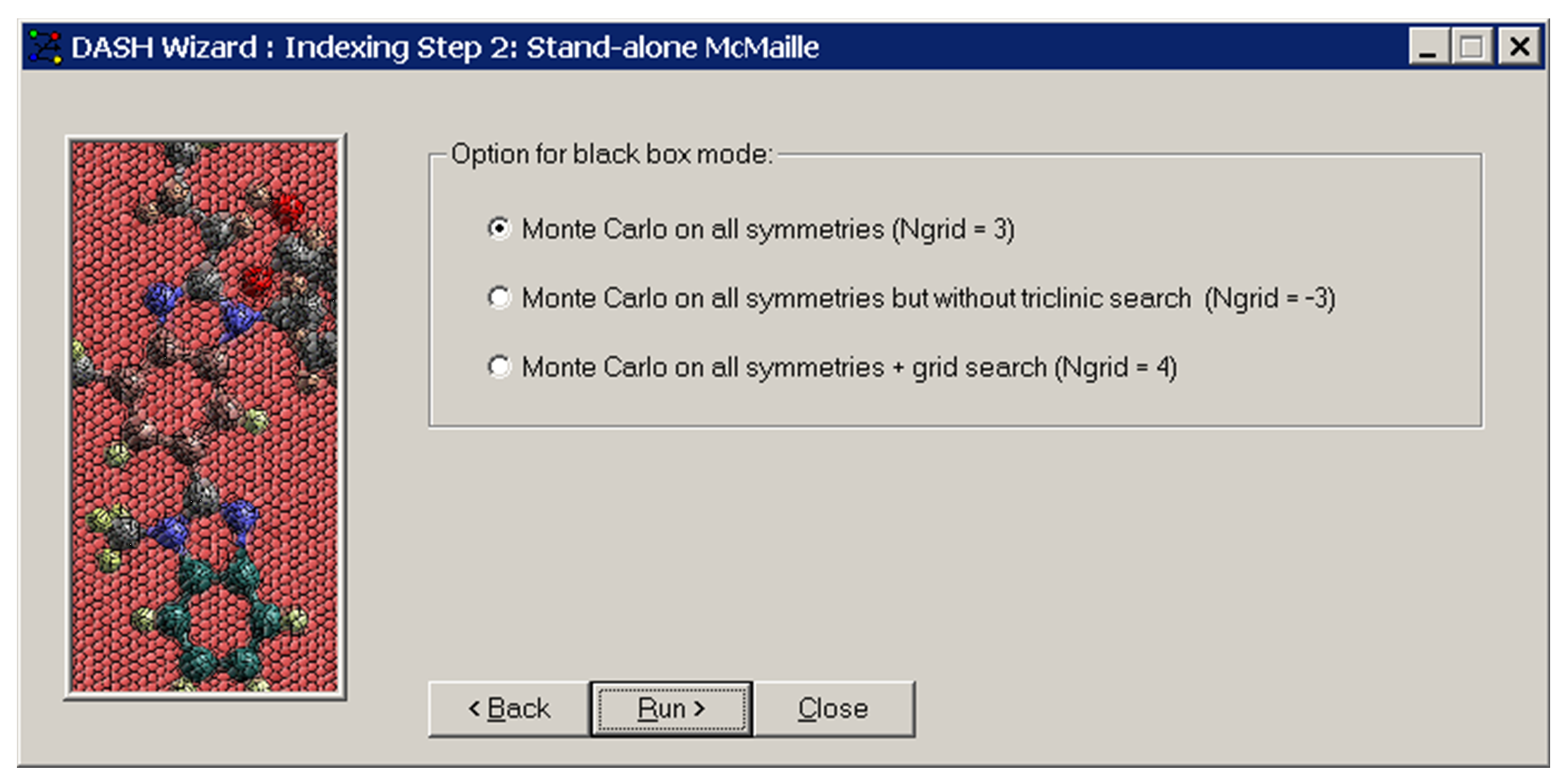
-
Select which group of symmetries you would like to explore and whether a grid search is required.
-
Indexing in the triclinic crystal system may take a long time with McMaille.
-
Click Run>.
-
Once McMaille has finished running, you will be prompted to type a character and press return. The results from the indexing will then be presented in a text window. Closing this window will return you to DASH where you can enter your chosen cell parameters into the Unit Cell Parameter wizard window (see Viewing Unit Cell Parameters).

-
Select the appropriate solution by selecting the button next to it in the Import column.
-
Clicking Next > will take you automatically to the Unit Cell Parameters wizard window.

-
Fill in details of the unit cell parameters and space group (see Viewing Unit Cell Parameters).
-
The unit cell parameters can also be read in at this point from a crystal structure file by clicking on the Browse... button.
-
Click Next >.

-
Proceed with peak selection for indexing as described in (see Selecting Peaks for Indexing).
-
Click Next >.
Pawley refinement is the next step (see Pawley Fitting) followed by structure solution (see Structure Solution).