PreliminaryProfileInspection
Unfortunately, it is not possible to guess whether a structure will solve just by looking at the diffraction data. However, a preliminary visual inspection of the data is always worthwhile, as it may give clues about possible problems. Things to look out for are:
-
Signal-to-noise ratio (see Signal-to-Noise Ratio).
-
ESDs (see Initial Assessment of ESDs).
-
Background shape (see Initial Assessment of Background Shape).
-
Peak shapes (see Initial Assessment of Peak Shapes).
-
Balance of peak intensities (see Patterns Dominated by a Few Strong Peaks) and (see Flattened Peak Tops).
-
Useful 2θ range (see Initial Assessment of Useful 2θ Range).
When you input a diffraction data file to DASH, the default display is of the complete data set, over the full range of 2θ. There are several methods for examining chosen areas of the data set.
-
The simplest way to zoom is to use the left mouse button; ensure that you are in Zoom mode (this is the default mode) by selecting Default from the Mode menu, or depressing the icon on the menu bar.
-
Click and hold the left mouse button and drag out a rectangle around the area that you want to zoom in on.
-
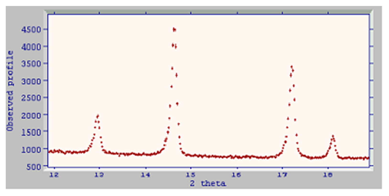
To zoom out, simply select the Home key on the keyboard. This example shows the effect of zooming in on two peaks that lie just either size of 10° 2θ. You will see that DASH plots both the intensity and the error bars.

-
A useful keyboard short-cut for zooming in on the 2θ axis is to select **Shift -**↑. Selecting **Shift -**↓ will zoom out on the 2θ axis.
-
A useful command to re-scale the intensity axis to the maximum peak height in the selected range is to select Ctrl - ↑.
To zoom out and display the full data set, simply select the Home key on the keyboard.
You can use the left and right cursor keys to move up left or right through the data in 2θ, (the horizontal axis). Selecting the Shift key in conjunction with the left or right cursor keys allows the same movement, but with a smaller step size. The up and down cursor keys allow you to move the window up and down in the intensity range (the vertical axis).
-
How easy is it to distinguish the Bragg peaks from the background? Obviously, the noisier the data, the less certain we can be of obtaining a definitive crystal structure.
-
The following examples should help give you some idea of what good, average and poor quality diffraction patterns look like:
This is synchrotron data from a nicely crystalline sample, with an incident wavelength of 0.6 Å. The background is low and the peak-to-background ratio is excellent, even at high angles. Individual ESDs of each point (displayed as vertical bars) are relatively small, showing that data have been collected for a sufficiently long time:


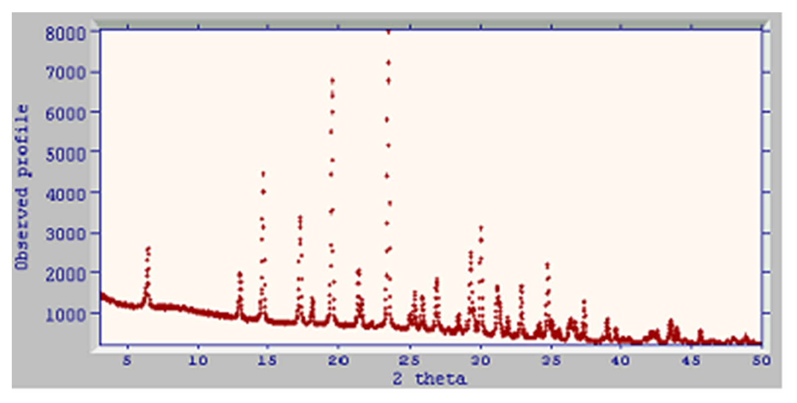
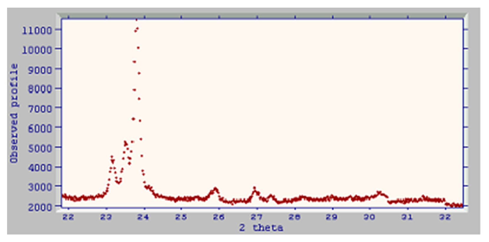
This is laboratory data (1.7889 Å wavelength) for a nicely crystalline sample (data by permission of Dr. L. Smrcok). The background counts are higher and the profile generally noisier than the example synchrotron pattern, but the background-to-noise ratio is still reasonable. The profile is significantly worse than the synchrotron example at high angle, but peaks are still sufficiently well-defined to produce useful information for structure solution:
This is laboratory data (1.54056 Å wavelength) for a rather poorly crystalline sample (data by permission of Dr. J. P. Attfield), the peaks are fairly broad and background is high, with little diffracted intensity beyond about 25o:
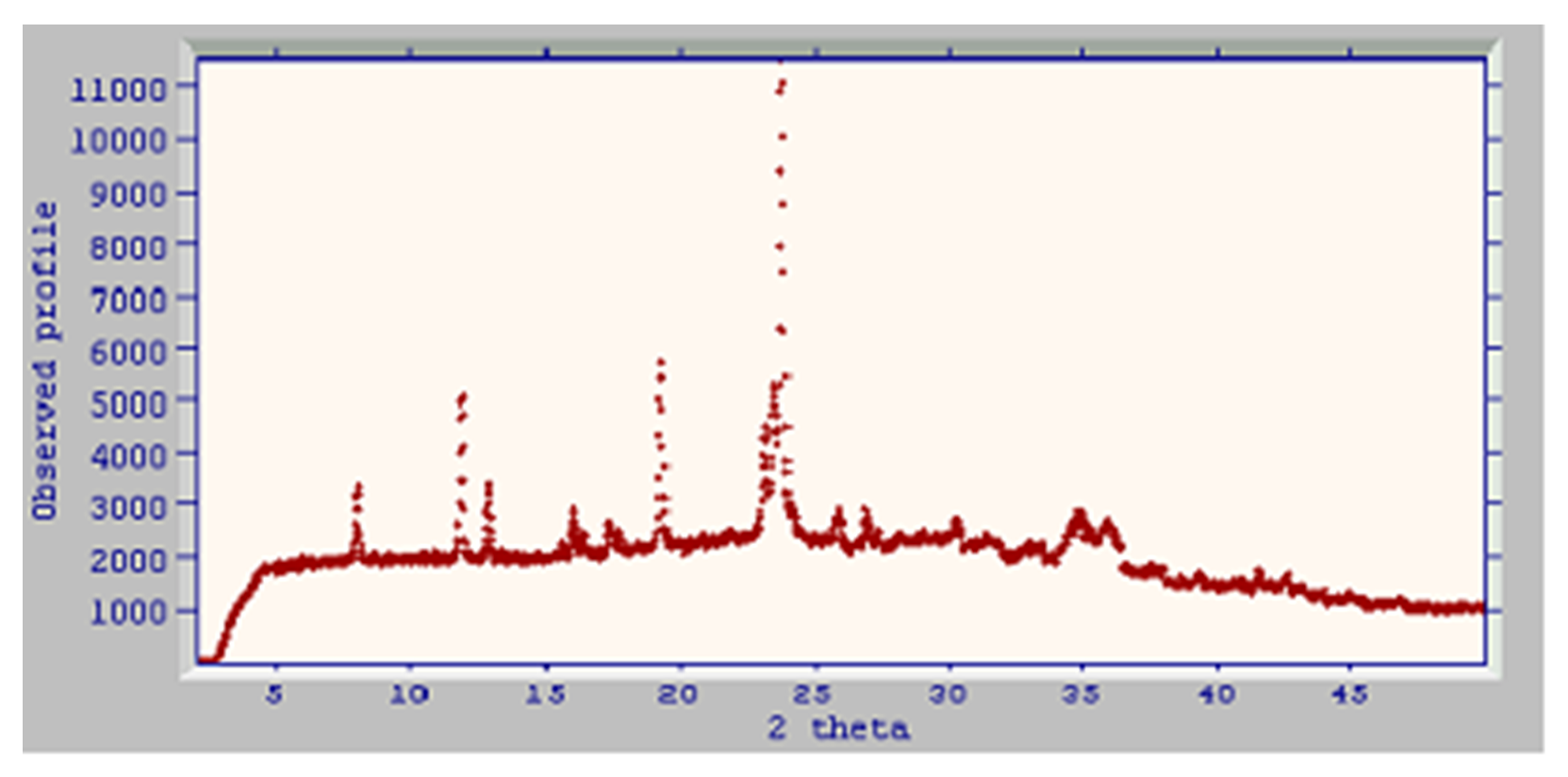
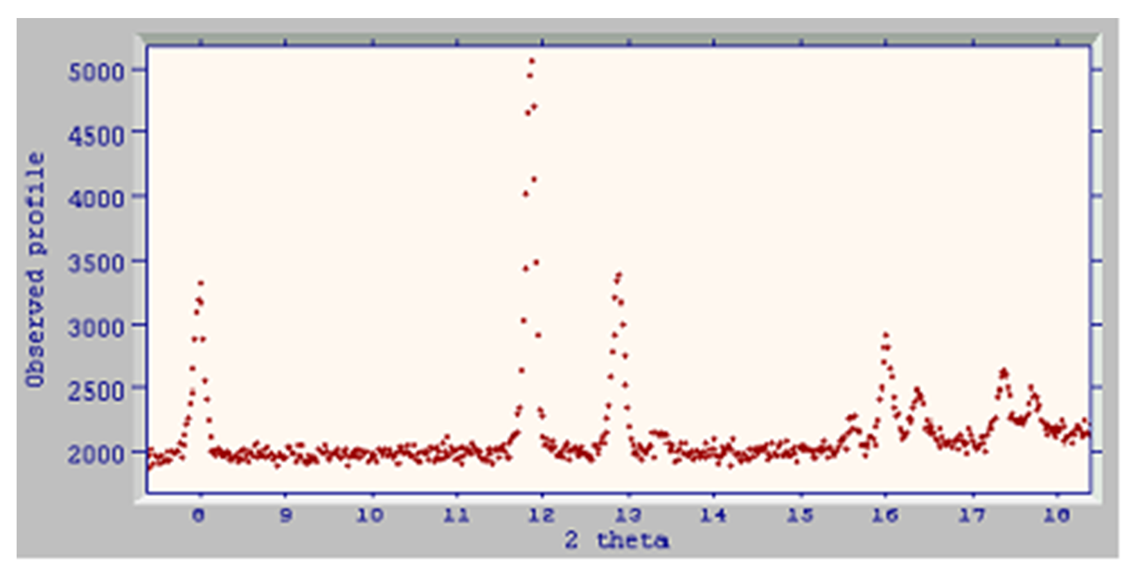
Note: The above data were actually sufficient to solve a problem involving 7 variable torsion angles. Remember that weak peaks, provided that they are sufficiently well determined, are just as powerful a constraint on the solution as strong peaks.
-
The error bars on the data points should look similar to those shown in the example profiles. If they look significantly bigger, then there could be a problem with the ESDs.
-
If you have been given a data set and you suspect that the ESDs are incorrect, then you can always replace them with the square roots of the counts, or delete them from the input file and let DASH calculate them.
-
Backgrounds may be largely flat, sloping, or rising-and-falling, as illustrated in the example profiles.
-
During data input, a Monte Carlo background estimation routine gives you the chance to fit and remove the background. You should normally use this background removal option.
-
During Pawley fitting, a second order polynomial is then sufficient to represent the background. If you did not take the background subtraction option, then a higher order polynomial will be used. The more complex the background, the more terms might have to be used in this polynomial.
DASH is able to fit the majority of peak shapes that you will encounter in diffraction from organic compounds, including asymmetry at low angles due to axial divergence.
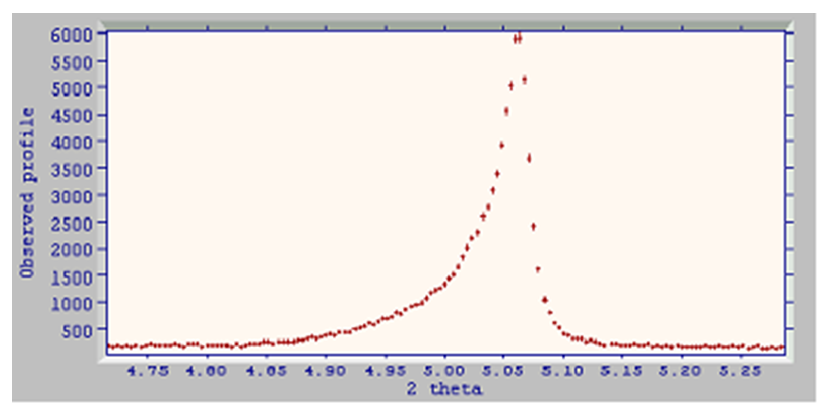
Asymmetry due to axial divergence at low angle:
Symmetric peaks at moderate resolution:

-
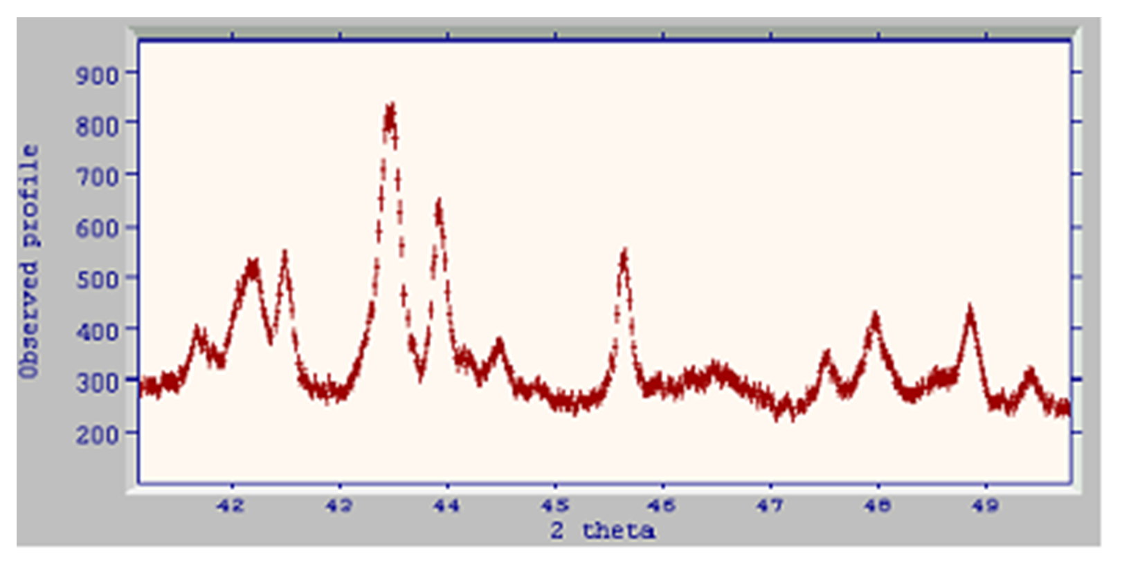
When visually assessing a diffraction pattern, it is useful to remember that, at low angles, peaks appear broadened by asymmetry. At high angles, peaks begin to overlap. Thus, it is probably best to assess the overall peak sharpness from the low to mid-range section of the diffraction pattern, where the probability of diffraction peaks being the result of individual Bragg reflections is much higher than at high angle.
-
Sharp diffraction peaks are obviously preferable, because the sharper the peaks, the less overlap there will be between adjacent peaks in the pattern.
-
The most obvious reason for broad peaks in a diffraction pattern is that the compound under study possesses intrinsically broad peaks. Frequently, recrystallisation of the sample can improve matters, but normally we are stuck with the sample as-is and must accept the broader peaks.
-
It is always possible that peaks that appear broad are actually doublets (i.e. closely spaced pairs of peaks).
-
If any of the peaks are noticeably sharper than the others, this can indicate hkl-dependent line broadening (i.e. some classes of reflections are sharper than others). If only relatively few reflections are affected and the broadening is not excessive, this will not preclude structure solution.
If your diffraction pattern is dominated by just a few very strong peaks, the following possibilities exist:
-
The distribution of intensities may be correct. For example, this type of pattern will result if a planar molecule is lying so that the bulk of its scattering power is concentrated within a few hkl planes.
-
Weak peaks, provided that they are sufficiently well determined, are just as powerful a constraint on the structure solution as strong peaks.
-
The distribution of intensities may be indicative of preferred orientation, i.e. the crystallites in the powder sample were not randomly oriented with respect to the incident radiation, but tended to be aligned along a certain direction. Preferred orientation is not usually a big problem if transmission capillary data has been collected. Whilst, in principle, the direction and extent of preferred orientation within the sample can be determined as part of the structure solution process, in the current version of DASH only the extent of the preferred orientation can be optimised during the simulated annealing.
-
In rare cases, a large peak may turn out to be an instrumental artefact, e.g. a spike in the detector electronics. Such rogue points can normally be edited out by hand.
If strong peaks in your diffraction pattern appear to have flattened tops, it is likely that the detector has been saturated during the data collection. If the flattening has seriously truncated the height of the peak, you will not be able to obtain an accurate intensity value for the peak during Pawley fitting.
-
A simple rule of thumb for assessing the useful data range obtained in a powder diffraction experiment is to take all the data from the lowest 2θ value to the highest value at which Bragg peaks are still clearly discernible from the background.
-
There is little point in including data in the Pawley refinement that is above the useful range; it will merely slow the refinement down without adding useful information. In extreme cases, it may actually hinder structure solution, as unreliable information has been introduced into the problem.
-
Structure solution does not normally require as much data as structure refinement. Diffraction data up to 1.5 Å resolution are normally sufficient for a successful structure solution, though in many cases, data to 2.0 Å or even lower resolution will suffice.
-
DASH will handle up to a total of around 600 refinable intensities during the Pawley fitting process.